The Wave Equation

Chem 3240 · Lecture 2.2

Davit Potoyan

The classical wave equation

\frac{\partial^2 u}{\partial x^2} = \frac{1}{v^2}\frac{\partial^2 u}{\partial t^2}

• Linear, second order in x and t
• General solution f(x - vt) + g(x + vt)
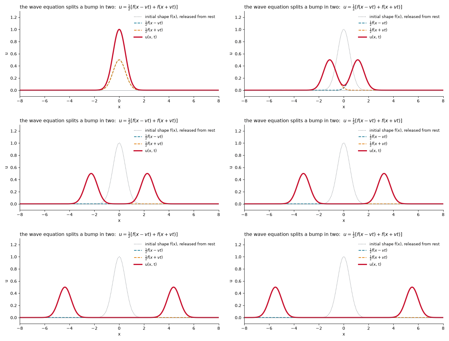
• A bump released from rest splits in two

Clamped ends change everything

1. Boundary conditions

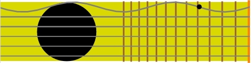
u(0,t) = 0, \qquad u(L,t) = 0

2. Separation of variables

u(x,t) = X(x)\,T(t)

3. Superposition

u = \sum_n c_n\, u_n

Step 1: separate the variables

Plug u = X(x)T(t) into the wave equation and divide by XT:

\frac{1}{v^2\,T}\frac{d^2T}{dt^2} = \frac{1}{X}\frac{d^2X}{dx^2} = K

• Left side depends only on t, right side only on x: both equal one constant K

One PDE becomes two ODEs

\frac{d^2X}{dx^2} - KX = 0, \qquad \frac{d^2T}{dt^2} - Kv^2\,T = 0

Step 2: turn the ODE into algebra

Trial function: every derivative of e^{rx} returns a multiple of e^{rx}

X = e^{rx} \quad\Rightarrow\quad \frac{d^2X}{dx^2} = r^2\,e^{rx}

Plug into X'' - KX = 0 and factor:

r^2 e^{rx} - K\,e^{rx} = \left(r^2 - K\right)e^{rx} = 0

r^2 = K \qquad\Rightarrow\qquad r = \pm\sqrt{K}

• e^{rx} is never zero, so the bracket must vanish: the differential equation became algebraic, two roots for two constants

Example: damped oscillator

Solve \dfrac{d^2y}{dt^2} + 2\beta\dfrac{dy}{dt} + \omega^2 y = 0 with the trial function e^{rt}.

r^2 + 2\beta r + \omega^2 = 0 \quad\Rightarrow\quad r = -\beta \pm \sqrt{\beta^2 - \omega^2}

\beta < \omega:\; r = -\beta \pm i\omega_d, \quad y = e^{-\beta t}\left[C_1\cos\omega_d t + C_2\sin\omega_d t\right]

\beta > \omega:\; r_1, r_2 \text{ real and negative}, \quad y = C_1 e^{r_1 t} + C_2 e^{r_2 t}

• \omega_d^2 = \omega^2 - \beta^2: the sign of the discriminant decides between oscillation and plain decay

Complex roots oscillate, real roots decay

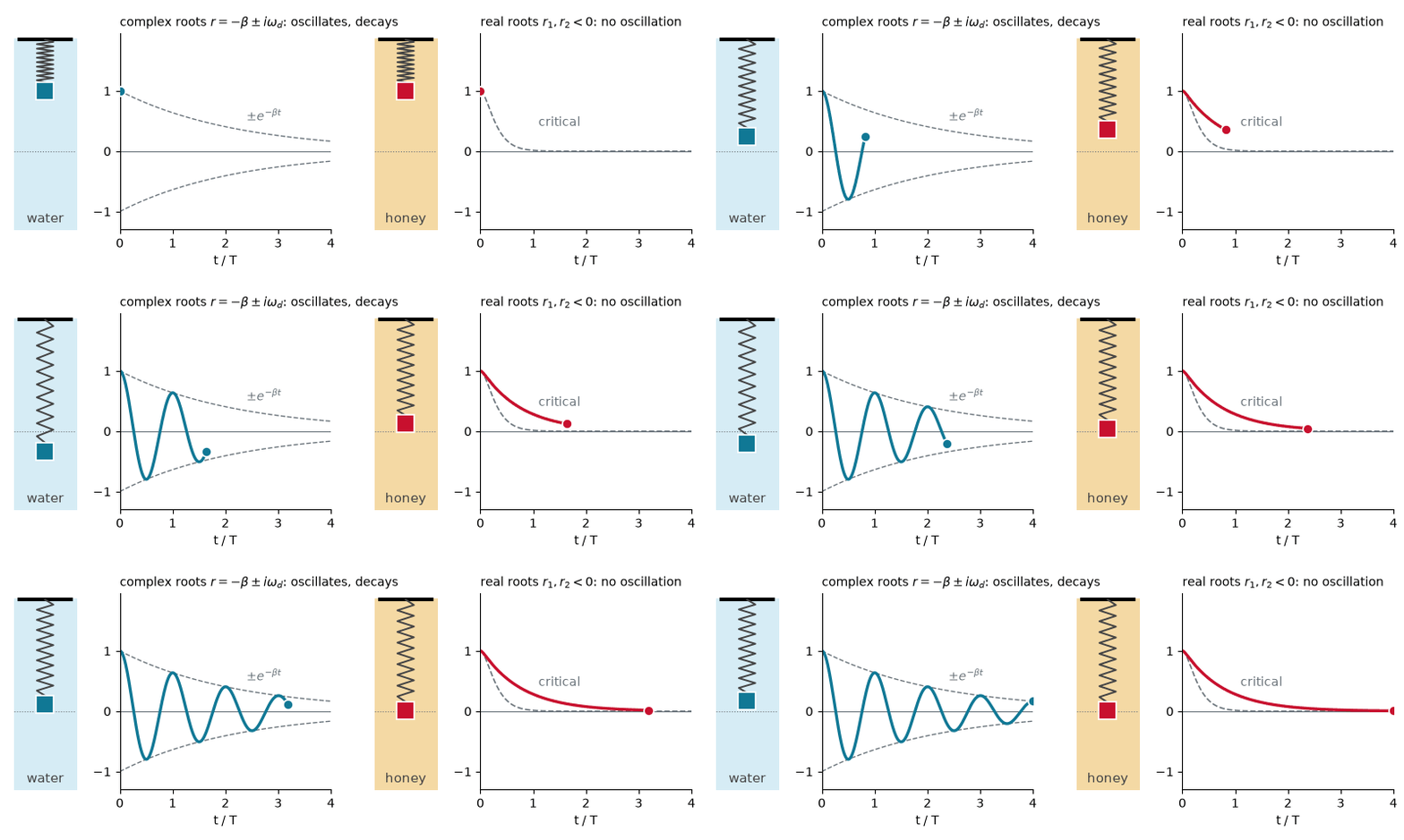
• Imaginary part of r sets the frequency, real part sets the decay
• The same test is coming for X'' - KX = 0: the sign of K picks the root type

Step 2: the sign of K decides

K = \beta^2 > 0: real roots

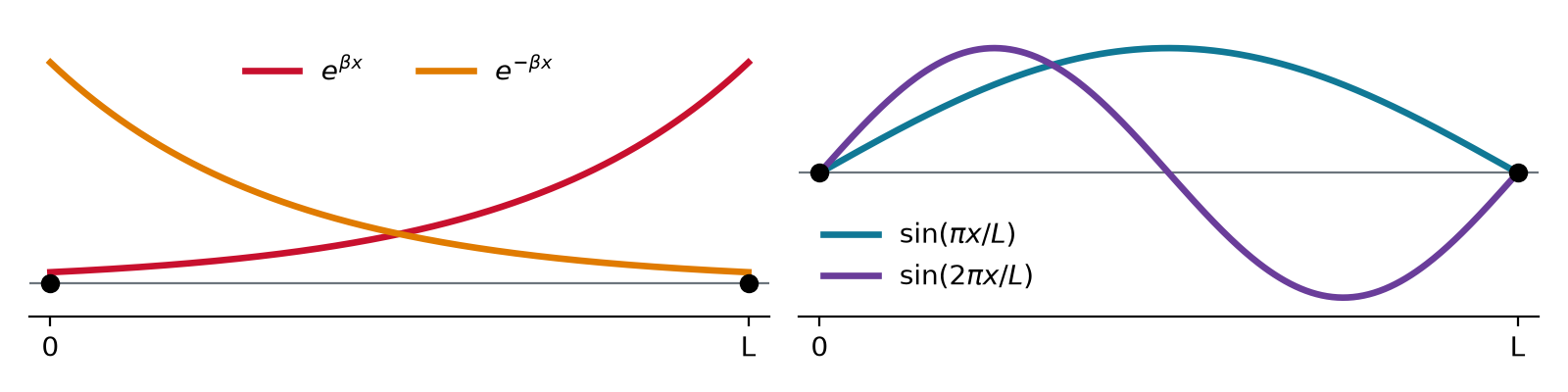
X = c_1e^{\beta x} + c_2e^{-\beta x}

• X(0) = X(L) = 0 forces c_1 = c_2 = 0
• No motion, no music

K = -\beta^2 < 0: imaginary roots

X = A\cos\beta x + B\sin\beta x

• X(0) = 0 gives A = 0
• X(L) = 0 needs \sin\beta L = 0

Boundary conditions quantize

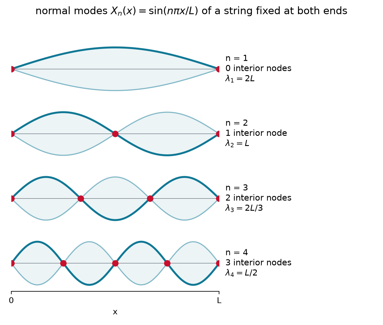
\sin\beta L = 0 only at multiples of \pi, so \beta_n = n\pi/L with n = 1, 2, 3, \ldots

X_n(x) = B_n\sin\frac{n\pi x}{L}

• An integer appeared from a boundary condition
• \lambda_n = 2L/n: half-wavelengths must fit
• Mode n has n - 1 nodes

The time part

• No boundary conditions on t: time marches on
• Insert K = -\beta_n^2: the harmonic oscillator equation

\frac{d^2T}{dt^2} + \beta_n^2 v^2\,T = 0 \quad\Longrightarrow\quad T_n(t) = A_n\cos(\omega_n t + \phi_n), \qquad \omega_n = \frac{n\pi v}{L}

• Each mode has its own frequency, an integer multiple of the fundamental
• A_n and \phi_n are not fixed yet: they wait for the initial conditions

Step 3: the full solution

u(x,t) = \sum_{n=1}^{\infty} A_n \sin\left(\frac{n\pi x}{L}\right)\cos(\omega_n t + \phi_n), \qquad \omega_n = \frac{n\pi v}{L}

• Modes X_n: a property of the string (length, clamps)
• Amplitudes and phases: a property of the pluck
• Every possible motion of the string is in this sum

Modes combine

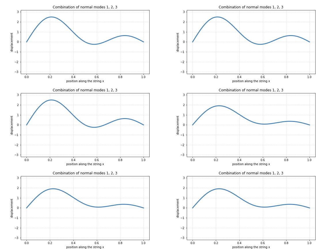
• A single mode is a standing wave with fixed nodes; a sum of modes sloshes, because each mode runs at its own frequency

Example: mode frequencies of a string

A string with L = 0.50 m carries waves at v = 200 m/s. Find the wavelengths and frequencies of the first three modes.

\lambda_n = \frac{2L}{n} = 1.00,\; 0.50,\; 0.33\ \text{m}

\nu_n = \frac{v}{\lambda_n} = n\frac{v}{2L} = 200,\; 400,\; 600\ \text{Hz}

• Only L and v enter: the string fixes the allowed frequencies, the pluck fixes how loud each one is

The pluck sets the amplitudes

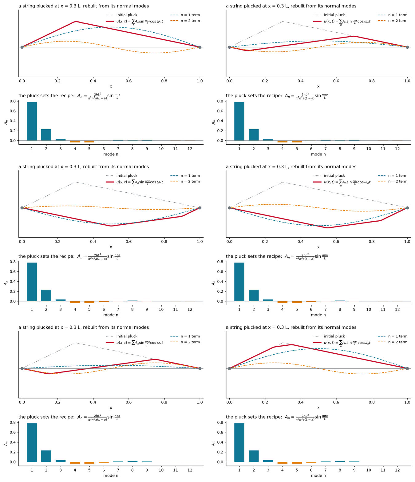
Released from rest: \phi_n = 0 and f(x) = \sum_n A_n \sin\frac{n\pi x}{L}

A_n = \frac{2}{L}\int_0^L f(x)\sin\frac{n\pi x}{L}\,dx

• Multiply by one mode and integrate: orthogonality kills every other term
• A mode with a node at the pluck stays silent

Live: move the pluck

Pluck position a sets the mix of harmonics: A_n \propto \sin(n\pi a/L)\,/\,n^2

viewof apos = Inputs.range([0.05, 0.95], {step: 0.01, value: 0.3, label: "pluck position a / L"})

{
  const N = 12;
  const An = d3.range(1, N + 1).map(n => ({n, A: 2 * Math.sin(n * Math.PI * apos) / (Math.PI**2 * n*n * apos * (1 - apos))}));
  const xs = d3.range(0, 1.0001, 0.005);
  const shape = xs.map(x => ({x, y: x < apos ? x / apos : (1 - x) / (1 - apos)}));
  const rebuilt = xs.map(x => ({x, y: d3.sum(An, d => d.A * Math.sin(d.n * Math.PI * x))}));
  const left = Plot.plot({width: 580, height: 320, x: {label: "x / L"}, y: {domain: [-0.2, 1.2], label: "u / h"},
    marks: [Plot.ruleY([0], {stroke: "#ccc"}),
            Plot.line(shape, {x: "x", y: "y", stroke: "#6c757d", strokeDasharray: "4,4"}),
            Plot.line(rebuilt, {x: "x", y: "y", stroke: "#C8102E", strokeWidth: 2.5})]});
  const right = Plot.plot({width: 520, height: 320, x: {label: "mode n", tickFormat: d => d}, y: {domain: [-0.35, 0.9], label: "Aₙ / h"},
    marks: [Plot.ruleY([0], {stroke: "#ccc"}),
            Plot.barY(An, {x: "n", y: "A", fill: d => d.A >= 0 ? "#107895" : "#e07b00"})]});
  return html`<div style="display:flex; gap: 24px; align-items: flex-start">${left}${right}</div>`;
}

md`Dashed: the pluck. Red: the first 12 modes added up. Silent modes at this pluck: **${d3.range(1, 13).filter(n => Math.abs(Math.sin(n * Math.PI * apos)) < 0.02).join(", ") || "none below n = 12"}**`

Two dimensions: degeneracy

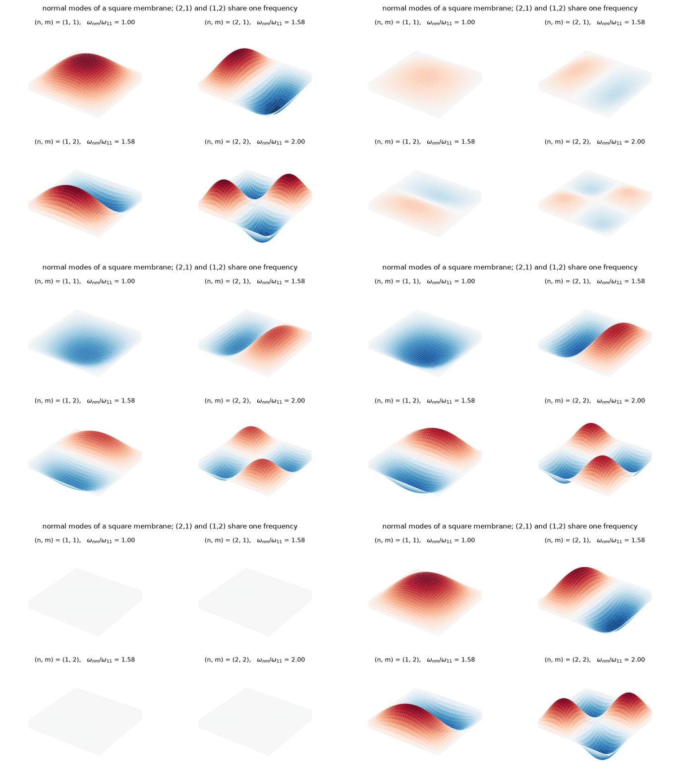
u = X(x)\,Y(y)\,T(t): two integers n, m

\omega_{nm} = v\pi\sqrt{\frac{n^2}{a^2} + \frac{m^2}{b^2}}

• Frequencies are not integer multiples: a drum has no pitch
• Square: (2,1) and (1,2) share \omega, they are degenerate
• Degeneracy comes from symmetry

Same recipe, next chapter

classical string	quantum particle in a box
u_{xx} = u_{tt}/v^2	-\frac{\hbar^2}{2m}\Psi_{xx} + V\Psi = i\hbar\Psi_t
u = X(x)\,T(t)	\Psi = \psi(x)\,e^{-iEt/\hbar}
X(0) = X(L) = 0	\psi(0) = \psi(L) = 0
modes \sin(n\pi x/L)	states \sin(n\pi x/L)
\omega_n \propto n	E_n \propto n^2
pluck sets A_n	state sets c_n

• Boundary conditions make integers, orthogonality extracts amplitudes

Takeaway

Separation of variables turns the wave equation into ODEs, boundary conditions turn the ODEs into quantized normal modes, and initial conditions decide how much of each mode is present. Chapter 3 runs the same recipe on the Schrödinger equation.