Operators 1: Matrices and Dirac Notation

Chem 3240 · Lecture 3.5

Davit Potoyan

The rules of the game

postulate lecture
1 the state is a wavefunction \psi; \lvert\psi\rvert^2 is the probability density 3.1
2 every observable is a linear Hermitian operator 3.5, 3.5b
3 a measurement returns an eigenvalue a_n and leaves the state \phi_n 3.6
4 outcome a_n has probability \lvert\langle\phi_n\vert\psi\rangle\rvert^2 3.6
5 the state evolves by i\hbar\,\partial\Psi/\partial t = \hat{H}\Psi 3.7
  • Today: a change of viewpoint. Functions become vectors, operators become matrices
  • Next lecture: which matrices may stand for an observable (Hermitian), and what if two do not commute

Operators must be linear

\hat{A}\,(c_1\psi_1 + c_2\psi_2) = c_1\,\hat{A}\psi_1 + c_2\,\hat{A}\psi_2

  • Superposition demands it: if \Psi_1 and \Psi_2 are states, so is their sum
  • Linear: x, d/dx, \hat{H}. Not linear: f^2, \sqrt{f}, \ln f
  • Quick test: a linear operator turns 2f into 2\hat{A}f; squaring gives 4f^2

A matrix turns and stretches arrows

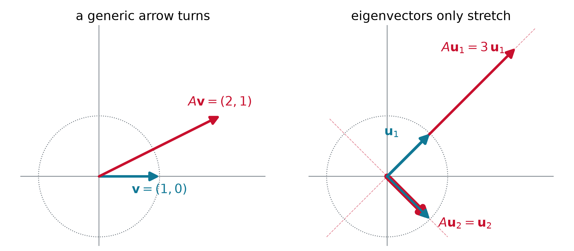
\begin{pmatrix} 2 & 1 \\ 1 & 2 \end{pmatrix}\begin{pmatrix} 1 \\ 0 \end{pmatrix} = \begin{pmatrix} 2 \\ 1 \end{pmatrix}\ \text{turned}, \qquad\qquad \begin{pmatrix} 2 & 1 \\ 1 & 2 \end{pmatrix}\begin{pmatrix} 1 \\ 1 \end{pmatrix} = 3\begin{pmatrix} 1 \\ 1 \end{pmatrix}\ \text{only stretched}

  • An eigenvector keeps its direction, A\mathbf{v} = \lambda\mathbf{v}: the same shape as \hat{A}\phi = a\phi

Live: hunt for the eigenvectors

Example: eigenvalues of a 2×2 by hand

A\mathbf{v} = \lambda\mathbf{v}\ \text{ with }\ \mathbf{v} \neq 0 \qquad\Longleftrightarrow\qquad \det(A - \lambda I) = 0

Find the eigenvalues and eigenvectors of A = \begin{pmatrix} 2 & 1 \\ 1 & 2 \end{pmatrix}.

\det\begin{pmatrix} 2-\lambda & 1 \\ 1 & 2-\lambda \end{pmatrix} = (2-\lambda)^2 - 1 = 0 \quad\Longrightarrow\quad \lambda = 3,\ 1

\lambda = 3: \mathbf{v} \propto (1, 1). \ \lambda = 1: \mathbf{v} \propto (1, -1). Check: 3 + 1 = 4 is the trace, 3 \times 1 = 3 the determinant.

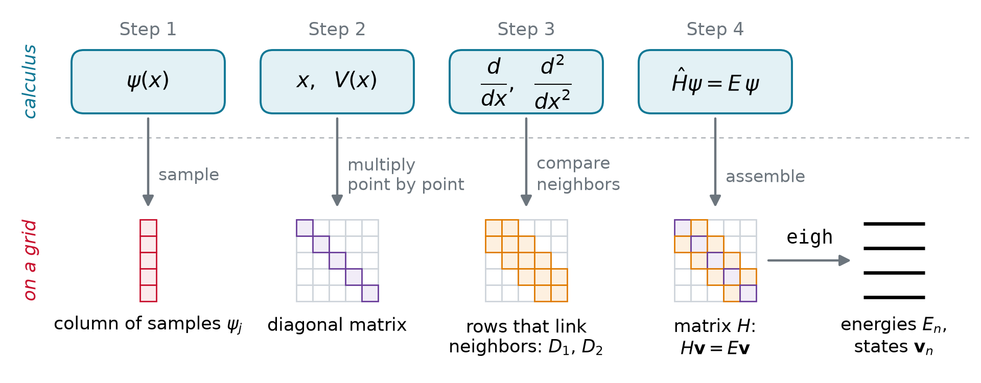
From operators to matrices: four steps

  • Each step swaps calculus (top) for what a computer can store (bottom)

One vector, two pictures

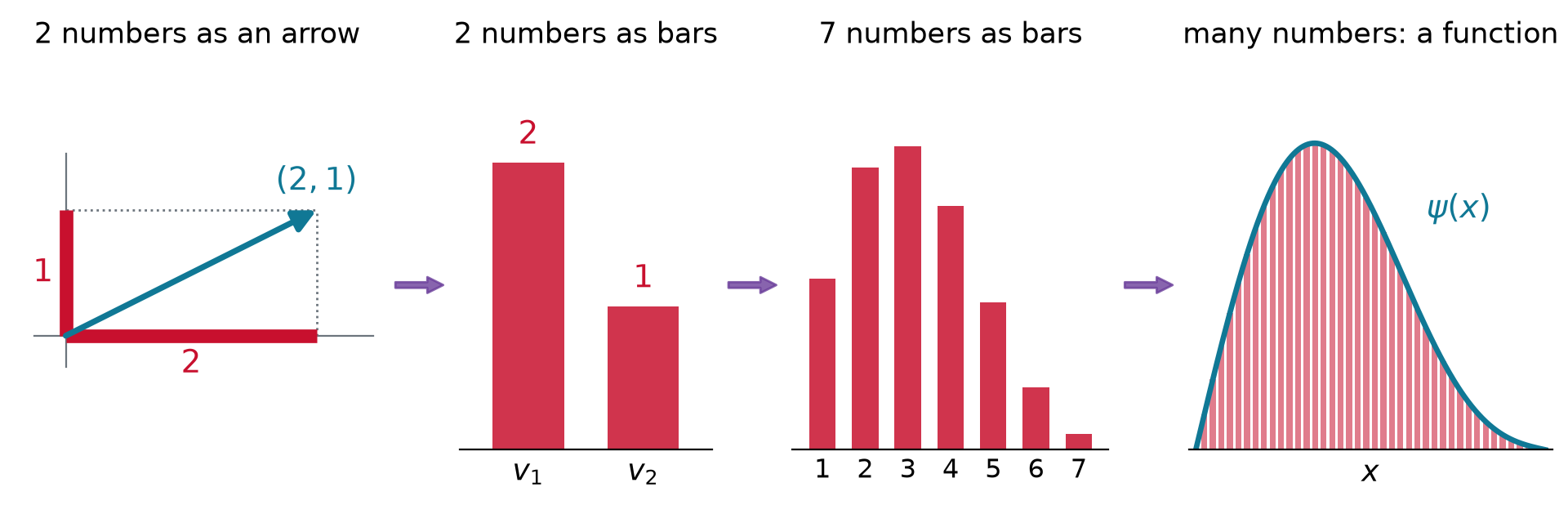
  • A vector is a list of numbers. An arrow shows two or three; bars show any number
  • Many bars trace a curve: a function is a vector, one component per point

A function becomes a vector

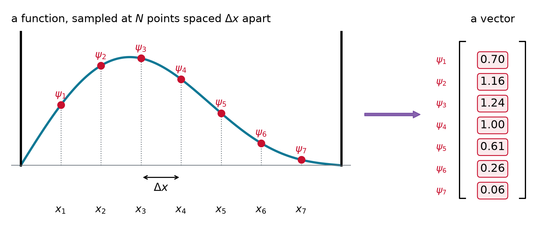
  • Sample at N points spaced \Delta x apart: \psi(x) \to (\psi_1, \psi_2, \dots, \psi_N), with \psi_j = \psi(x_j)
  • Integrals become sums: \int \phi^*\psi\,dx \;\to\; \sum_j \phi_j^*\,\psi_j\,\Delta x

Multiplying by x: a diagonal matrix

\hat{x}\,\psi \;\longrightarrow\; \begin{pmatrix} x_1 & 0 & 0 & 0 \\ 0 & x_2 & 0 & 0 \\ 0 & 0 & x_3 & 0 \\ 0 & 0 & 0 & x_4 \end{pmatrix} \begin{pmatrix} \psi_1 \\ \psi_2 \\ \psi_3 \\ \psi_4 \end{pmatrix} = \begin{pmatrix} x_1\psi_1 \\ x_2\psi_2 \\ x_3\psi_3 \\ x_4\psi_4 \end{pmatrix}

  • Each sample is multiplied by its own x_j: nothing off the diagonal
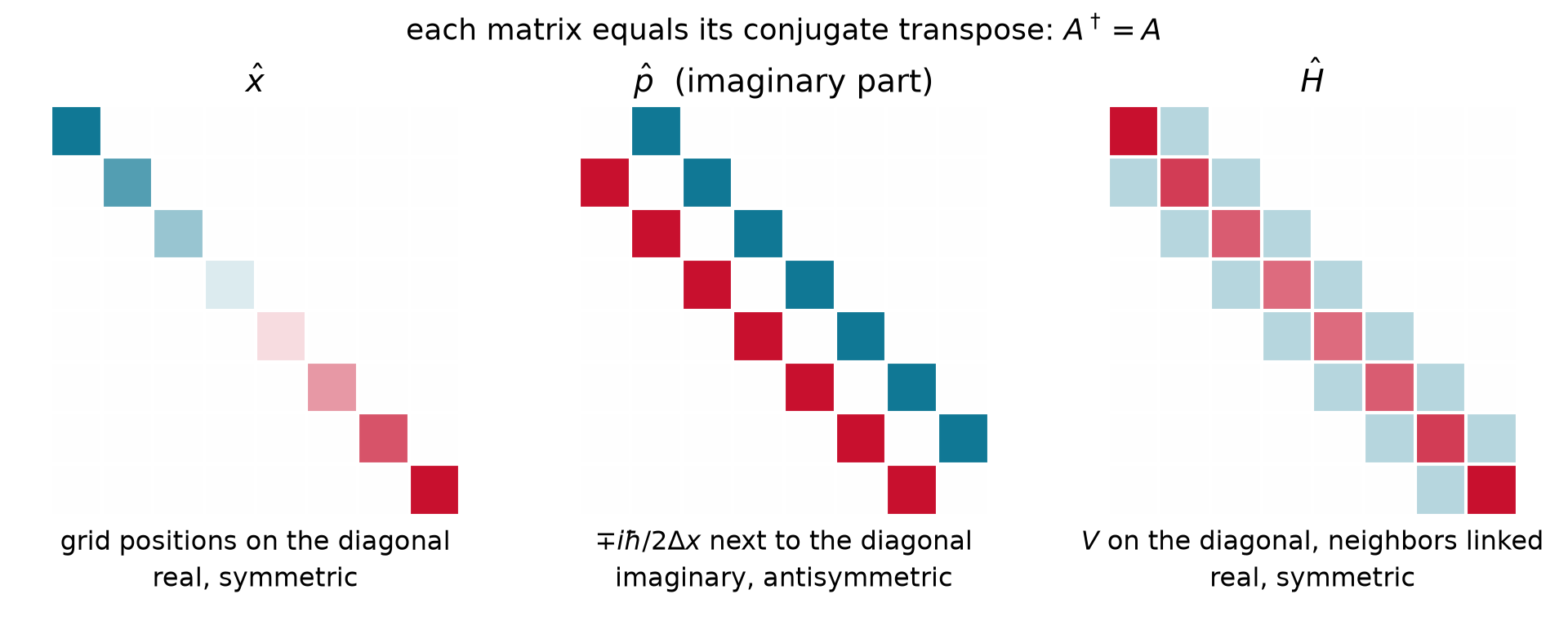
  • Any potential V(x) is diagonal the same way, with V(x_1), V(x_2), \dots on the diagonal

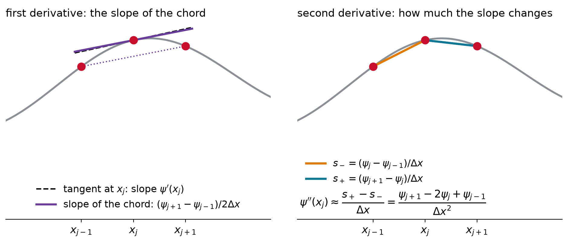
A derivative compares neighbors

\psi'(x_j) \approx \frac{\psi_{j+1} - \psi_{j-1}}{2\Delta x} \qquad\qquad \psi''(x_j) \approx \frac{s_+ - s_-}{\Delta x} = \frac{\psi_{j+1} - 2\psi_j + \psi_{j-1}}{\Delta x^2}

One formula, one matrix row

  • The curvature formula at point 2 uses three samples, with the numbers 1,\ -2,\ 1 in front of them:

\psi''(x_2) \approx \frac{1\cdot\psi_1 - 2\,\psi_2 + 1\cdot\psi_3}{\Delta x^2} = \frac{1}{\Delta x^2}\begin{pmatrix} 1 & -2 & 1 & 0 \end{pmatrix}\begin{pmatrix} \psi_1 \\ \psi_2 \\ \psi_3 \\ \psi_4 \end{pmatrix}

  • Row times column: multiply matching entries, then add them up
  • So the formula’s numbers are a row of a matrix. At point 3 the same numbers move one place right: (0,\ 1,\ -2,\ 1)

Derivatives as matrices

\begin{aligned} \frac{d}{dx} \;\to\; D_1 &= \frac{1}{2\Delta x}\begin{pmatrix} 0 & 1 & 0 & 0 \\ -1 & 0 & 1 & 0 \\ 0 & -1 & 0 & 1 \\ 0 & 0 & -1 & 0 \end{pmatrix} \\[6pt] \frac{d^2}{dx^2} \;\to\; D_2 &= \frac{1}{\Delta x^2}\begin{pmatrix} -2 & 1 & 0 & 0 \\ 1 & -2 & 1 & 0 \\ 0 & 1 & -2 & 1 \\ 0 & 0 & 1 & -2 \end{pmatrix} \end{aligned}

  • One row per grid point: the same formula each time, shifted one place to the right
  • Row 1 of D_2 gives (-2\psi_1 + \psi_2)/\Delta x^2: the formula with \psi_0 = 0, so the wall is built in
  • Momentum \hat{p} = -i\hbar\,D_1: -i\hbar/2\Delta x above the diagonal, +i\hbar/2\Delta x below

Example: the grid derivative of a plane wave

Apply the centered difference to the samples of a plane wave, \psi_j = e^{ikx_j}.

\frac{\psi_{j+1} - \psi_{j-1}}{2\Delta x} = \frac{e^{ik\Delta x} - e^{-ik\Delta x}}{2\Delta x}\,e^{ikx_j} = \frac{i\sin(k\Delta x)}{\Delta x}\,\psi_j \;\;\xrightarrow{\;k\Delta x\,\ll\,1\;}\;\; ik\,\psi_j

An eigenvector of the matrix, as e^{ikx} is an eigenfunction of d/dx. Momentum: \hbar\sin(k\Delta x)/\Delta x \approx \hbar k.

  • The grid works when there are many points per wavelength

The Hamiltonian is a matrix

H = -\frac{\hbar^2}{2m}D_2 + V = \begin{pmatrix} 2\varepsilon + V_1 & -\varepsilon & 0 & 0 \\ -\varepsilon & 2\varepsilon + V_2 & -\varepsilon & 0 \\ 0 & -\varepsilon & 2\varepsilon + V_3 & -\varepsilon \\ 0 & 0 & -\varepsilon & 2\varepsilon + V_4 \end{pmatrix}, \quad \varepsilon = \frac{\hbar^2}{2m\,\Delta x^2}

\hat{H}\psi = E\,\psi \quad\longrightarrow\quad H\mathbf{v} = E\mathbf{v}

  • \varepsilon is only a unit of energy: the constants in front of D_2, collected in one symbol
  • Potential on the diagonal; kinetic energy links neighbors through -\varepsilon (the Hückel picture, too)

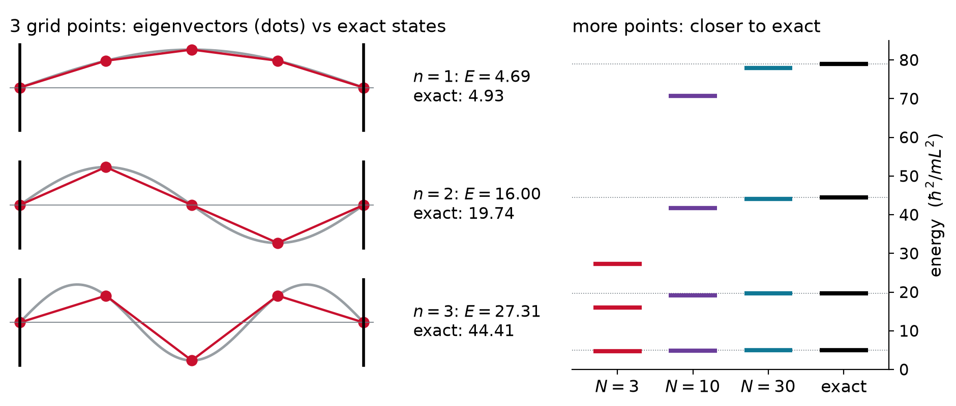
Example: a box with three grid points

Three interior points, \psi = 0 at the walls. Find the energies E = \lambda\,\varepsilon of \;H = \varepsilon\begin{pmatrix} 2 & -1 & 0 \\ -1 & 2 & -1 \\ 0 & -1 & 2 \end{pmatrix}.

Solve \det(H/\varepsilon - \lambda I) = 0 along the first row: each entry times the 2\times2 determinant left after crossing out its row and column, signs +\,-\,+:

\begin{aligned} &(2-\lambda)\underbrace{\big[(2-\lambda)^2 - 1\big]}_{\text{cross out row 1, column 1}} \;-\; (-1)\underbrace{\big[-(2-\lambda)\big]}_{\text{cross out row 1, column 2}} \;+\; 0 \\ &= (2-\lambda)\big[(2-\lambda)^2 - 2\big] = 0 \quad\Longrightarrow\quad \lambda = 2 - \sqrt{2},\ \ 2,\ \ 2 + \sqrt{2} \end{aligned}

Check the ground state by row times column

Sample the exact ground state \sin(\pi x/L) at the three points: \mathbf{v} = \big(\sin\tfrac{\pi}{4},\ \sin\tfrac{\pi}{2},\ \sin\tfrac{3\pi}{4}\big) \propto (1,\ \sqrt{2},\ 1). Is it an eigenvector of H?

\begin{pmatrix} 2 & -1 & 0 \\ -1 & 2 & -1 \\ 0 & -1 & 2 \end{pmatrix}\begin{pmatrix} 1 \\ \sqrt{2} \\ 1 \end{pmatrix} = \begin{pmatrix} 2 - \sqrt{2} \\ -1 + 2\sqrt{2} - 1 \\ -\sqrt{2} + 2 \end{pmatrix} = (2-\sqrt{2})\begin{pmatrix} 1 \\ \sqrt{2} \\ 1 \end{pmatrix}

Yes, with \lambda = 2 - \sqrt{2} (the middle entry 2\sqrt{2} - 2 is (2-\sqrt{2})\sqrt{2}). With \Delta x = L/4, \varepsilon = 8\hbar^2/mL^2 and E_1 = 4.69\,\hbar^2/mL^2, close to the exact 4.93.

More points, better answers

  • Eigenvectors are the exact states sampled on the grid; the levels converge from below

Five lines solve the Schrödinger equation

x = np.linspace(-8, 8, 400); dx = x[1] - x[0]
D2 = (np.eye(400, k=1) - 2*np.eye(400) + np.eye(400, k=-1)) / dx**2
H = -0.5 * D2 + np.diag(0.5 * x**2)      # spring: hbar = m = omega = 1
E, psi = np.linalg.eigh(H)
E[:4]                                    # 0.4999  1.4997  2.4993  3.4987
  • The same recipe with 400 points: the levels of a vibrating bond, \left(n + \tfrac{1}{2}\right)\hbar\omega
  • eigh is the eigensolver for Hermitian matrices. Why Hermitian? Coming up

Dirac notation: kets and bras

  • Ket \lvert\psi\rangle: the column of samples. Bra \langle\psi\rvert: the same numbers as a row, conjugated
  • A bra meeting a ket is an inner product, a single number:

\langle \phi \vert \psi \rangle = \sum_j \phi_j^*\,\psi_j\,\Delta x \;\;\longrightarrow\;\; \int \phi^*\,\psi\,dx

Why conjugate? Take \lvert\psi\rangle = \begin{pmatrix} 1 \\ i \end{pmatrix} and find \langle\psi\vert\psi\rangle.

\langle\psi\rvert = (1,\ -i), so \langle\psi\vert\psi\rangle = 1\cdot 1 + (-i)(i) = 2: a real, positive length squared. Without the conjugate, 1 + i^2 = 0: a nonzero vector of length zero. So a constant leaves a bra conjugated: \langle c\,\phi \vert \psi \rangle = c^*\langle \phi \vert \psi \rangle.

Sandwiches: matrix elements

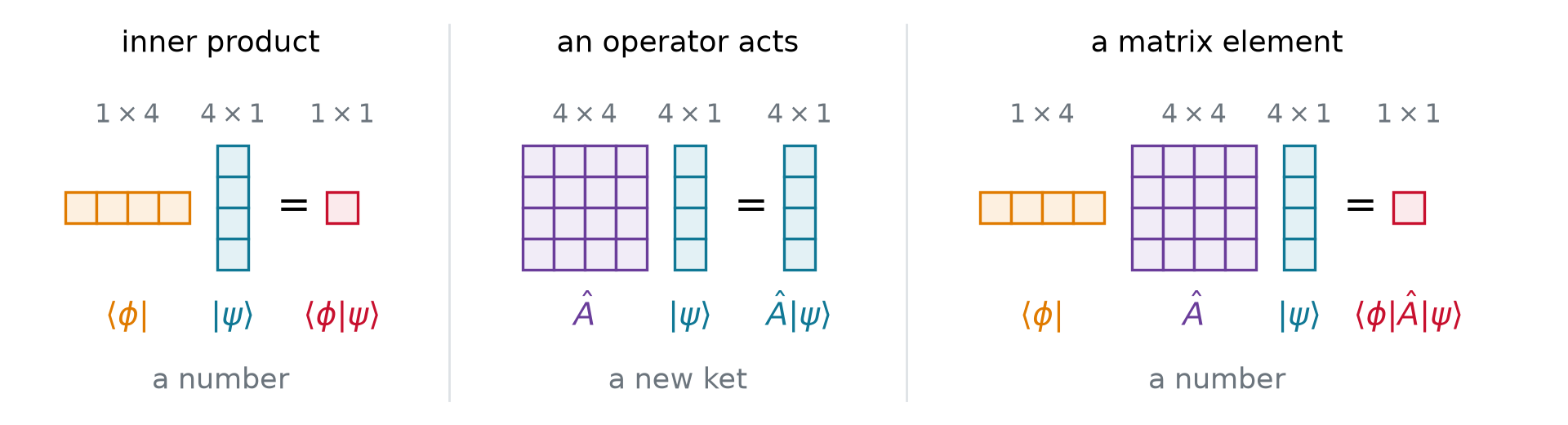
  • An operator acts on a ket: \hat{A}\lvert\psi\rangle is the matrix times the column
  • A bra in front turns it into a number, the matrix element:

\langle \phi \vert \hat{A} \vert \psi \rangle \;=\; \text{row} \times \text{matrix} \times \text{column} \;\;\longrightarrow\;\; \int \phi^*\,\hat{A}\psi\,dx

For A = \begin{pmatrix} 2 & 1 \\ 1 & 2 \end{pmatrix}, \mathbf{e}_1 = (1, 0) and \mathbf{e}_2 = (0, 1), compute \langle \mathbf{e}_1 \vert A \vert \mathbf{e}_2 \rangle.

A\,\mathbf{e}_2 = (1,\ 2), then \mathbf{e}_1 \cdot (1,\ 2) = 1 = A_{12}: sandwiching unit vectors picks out one entry of the matrix.

Count the shapes

  • Bra = row, operator = square, ket = column
  • Inner sizes must match; the outer sizes give the result: a number, or a new ket

Diagonalizing a Hamiltonian

  • The entries of a matrix depend on the axes; the operator does not. In perpendicular unit axes \mathbf{u}_1, \mathbf{u}_2, \dots each entry is a sandwich, A'_{mn} = \langle \mathbf{u}_m \vert A \vert \mathbf{u}_n \rangle

\langle \mathbf{u}_m \vert A \vert \mathbf{u}_n \rangle = \lambda_n\,\delta_{mn} \qquad \text{when } A\mathbf{u}_n = \lambda_n\mathbf{u}_n

  • In the axes of its eigenvectors a matrix is diagonal: eigenvalues on the diagonal, zeros elsewhere
  • Diagonalizing H means finding these axes; the diagonal lists the energies, {2 - \sqrt{2}},\ 2,\ {2 + \sqrt{2}} for the three-point box
  • E, U = np.linalg.eigh(H): the axes are the columns of U, and U.T @ H @ U is diagonal

Dirac notation: one language, three dialects

integral Dirac matrices (numpy)
inner product \int\phi^*\psi\,dx \langle\phi\vert\psi\rangle np.vdot(phi, psi) * dx
operator acts \hat{A}\psi(x) \hat{A}\lvert\psi\rangle A @ psi
matrix element \int\phi^*\hat{A}\psi\,dx \langle\phi\vert\hat{A}\vert\psi\rangle np.vdot(phi, A @ psi) * dx
eigenproblem \hat{A}\phi_n = a_n\phi_n \hat{A}\lvert n\rangle = a_n\lvert n\rangle a, phi = np.linalg.eigh(A)
new axes \int\phi_m^*\hat{A}\phi_n\,dx \langle \phi_m \vert \hat{A} \vert \phi_n \rangle U.conj().T @ A @ U * dx
  • The same objects in three dialects: integrals for functions, brackets on paper, matrices on a computer

Two matrix properties to watch

  • Mirror: each matrix equals its own conjugate transpose. Next lecture: Hermitian, which makes eigenvalues real
  • Order: for matrices AB \neq BA in general. Next lecture: commutators, and why x and p are never sharp together

Takeaway

Sample a function and it becomes a vector; every operator becomes a matrix. Position is diagonal, derivatives link neighbors, and the Hamiltonian is a matrix whose eigenvalues are the allowed energies. Dirac notation writes integrals and matrices in one language, and in the axes of its own eigenvectors a matrix is diagonal. Next: which matrices can be observables, and what happens when two of them do not commute.