Measurement: Eigenvalues and Expectation Values

Chem 3240 · Lecture 3.6

Davit Potoyan

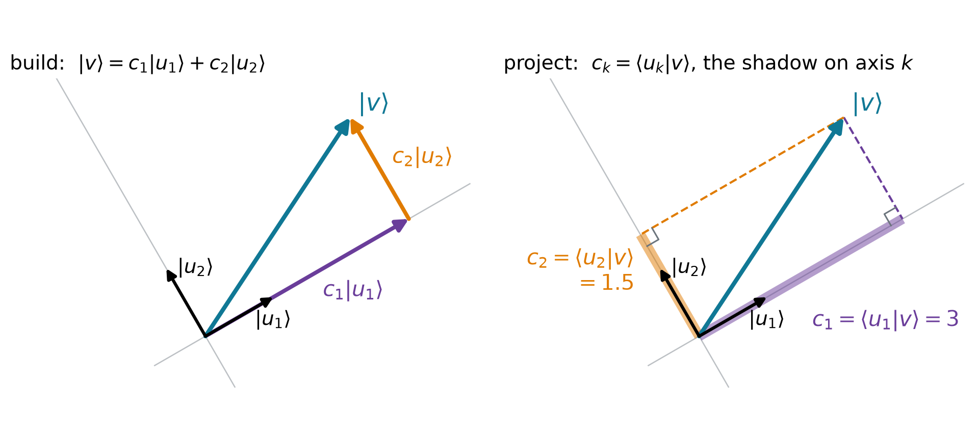
A vector: build it, then project

\langle u_1 \vert v\rangle = c_1\,\underbrace{\langle u_1 \vert u_1\rangle}_{1} + c_2\,\underbrace{\langle u_1 \vert u_2\rangle}_{0} = c_1

Example: components of a vector

Write \lvert v\rangle = (3, 4) in the tilted axes \lvert u_1\rangle = \tfrac{1}{\sqrt{2}}(1, 1) and \lvert u_2\rangle = \tfrac{1}{\sqrt{2}}(1, -1).

Each coefficient is a projection:

c_1 = \langle u_1 \vert v\rangle = \tfrac{3 + 4}{\sqrt{2}} = \tfrac{7}{\sqrt{2}}, \qquad c_2 = \langle u_2 \vert v\rangle = \tfrac{3 - 4}{\sqrt{2}} = -\tfrac{1}{\sqrt{2}}

\lvert v\rangle = c_1\lvert u_1\rangle + c_2\lvert u_2\rangle, \qquad c_1^2 + c_2^2 = \tfrac{49 + 1}{2} = 25 = \langle v \vert v\rangle

• Perpendicular unit axes: coefficients are projections, and their squares add up to the length squared

A function: the same two steps

• Build: the box states \lvert\psi_n\rangle are the axes, orthonormal, \langle \psi_m \vert \psi_n\rangle = \delta_{mn}

\lvert\psi\rangle = c_1\lvert\psi_1\rangle + c_2\lvert\psi_2\rangle + c_3\lvert\psi_3\rangle + \cdots

• Project: the bra \langle \psi_m\rvert picks out one coefficient, exactly as for the vector

\langle \psi_m \vert \psi\rangle = \sum_n c_n\,\underbrace{\langle \psi_m \vert \psi_n\rangle}_{\delta_{mn}} = c_m

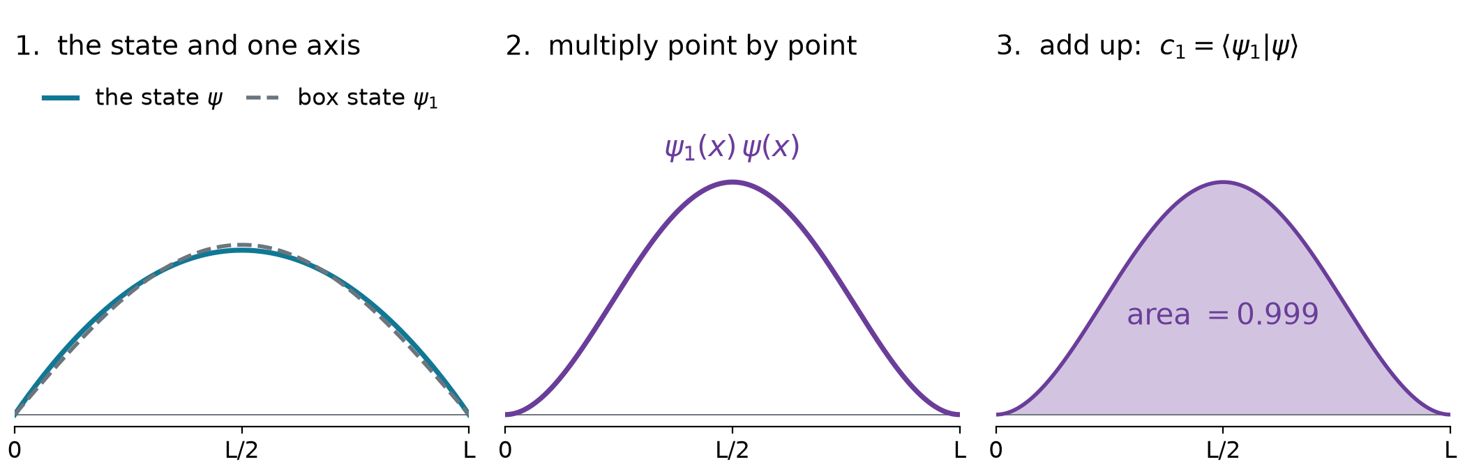
• The only new step: a bracket of two functions is an integral, \langle \psi_m \vert \psi\rangle = \int \psi_m^*\,\psi\,dx

One component, step by step

• The parabola \psi = \sqrt{30/L^5}\;x(L-x) looks almost like \psi_1, so its component along \psi_1 is almost 1: \ c_1 = 0.999

A component that vanishes

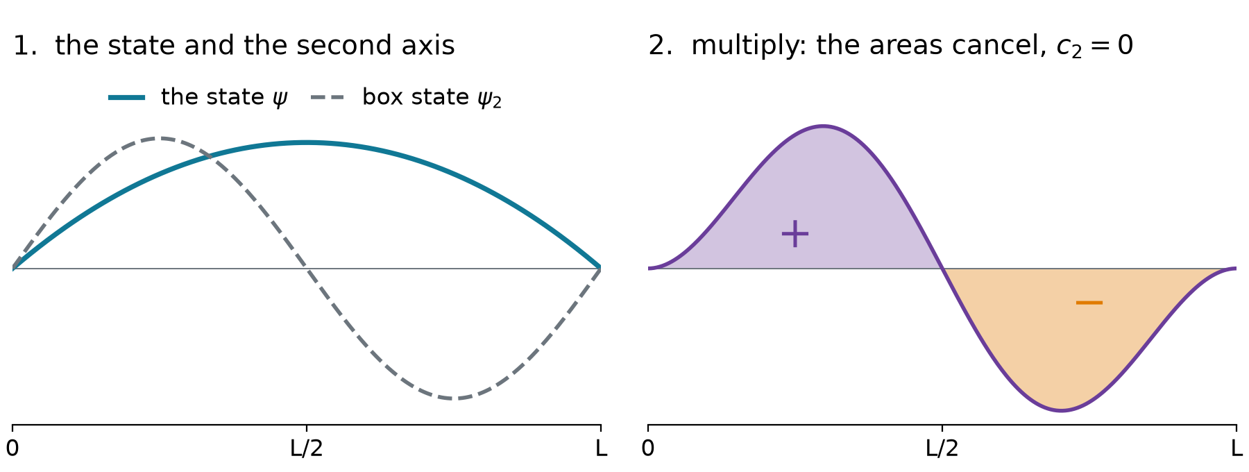
• \psi is symmetric about L/2, \psi_2 is antisymmetric: the two halves of the product cancel, so c_2 = 0
• The same happens for every even n: the parabola has no even components

One structure, two settings

	a vector in a plane	a function
axes	\lvert u_1\rangle, \lvert u_2\rangle	eigenfunctions \lvert\phi_1\rangle, \lvert\phi_2\rangle, \dots
orthonormal	\langle u_j \vert u_k\rangle = \delta_{jk}	\langle \phi_m \vert \phi_n\rangle = \delta_{mn}
build	\lvert v\rangle = \sum_k c_k\lvert u_k\rangle	\lvert\psi\rangle = \sum_n c_n\lvert\phi_n\rangle
project	c_k = \langle u_k \vert v\rangle	c_n = \langle \phi_n \vert \psi\rangle
the bracket	multiply matching components, add	multiply point by point, integrate

• Lecture 3.5’s grid made this literal: the integral is the dot product of the sampled values, times \Delta x

Eigenfunctions are coordinates

\lvert\psi\rangle = \sum_n c_n\,\lvert\phi_n\rangle, \qquad c_n = \langle \phi_n \vert \psi \rangle = \int \phi_n^*\,\psi\,dx

• The eigenfunctions \phi_n of an observable are the axes; c_n says how far \psi reaches along axis n
• Each c_n is a projection, found exactly as for the vector: multiply, then add up

Three one-line derivations

All three use only orthonormality, \langle \phi_m \vert \phi_n \rangle = \delta_{mn}:

\begin{aligned} \text{coefficient:}\quad & \langle \phi_m \vert \psi \rangle = \sum_n c_n\,\langle \phi_m \vert \phi_n \rangle = c_m \\[6pt] \text{normalization:}\quad & \langle \psi \vert \psi \rangle = \sum_m\sum_n c_m^*\,c_n\,\delta_{mn} = \sum_n \lvert c_n\rvert^2 = 1 \\[6pt] \text{average:}\quad & \langle \psi \vert \hat{A} \vert \psi \rangle = \sum_m\sum_n c_m^*\,c_n\,a_n\,\delta_{mn} = \sum_n \lvert c_n\rvert^2\,a_n \end{aligned}

• Same as the vector: squared components add up to one, the length of a normalized state

Example: how much ground state is in a parabola?

Expand \psi = \sqrt{30/L^5}\;x(L-x) in box states \psi_n = \sqrt{2/L}\,\sin(n\pi x/L).

Two integrations by parts:

c_n = \int_0^L \psi_n\,\psi\,dx = \frac{8\sqrt{15}}{(n\pi)^3}\ \ (n \text{ odd}), \qquad c_n = 0\ \ (n \text{ even: odd about } L/2)

\lvert c_1\rvert^2 = \frac{960}{\pi^6} = 0.9986, \qquad \lvert c_3\rvert^2 = 0.0014, \qquad \lvert c_5\rvert^2 = 0.0001

• A smooth, spread-out state is almost all ground state

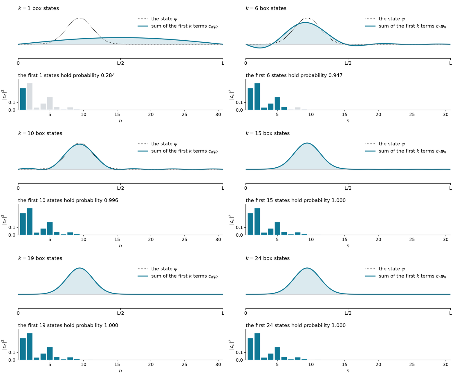
A narrow state needs many eigenstates

• Sharp features need short wavelengths, high n: about ten states for a packet 0.045\,L wide

A measurement returns an eigenvalue

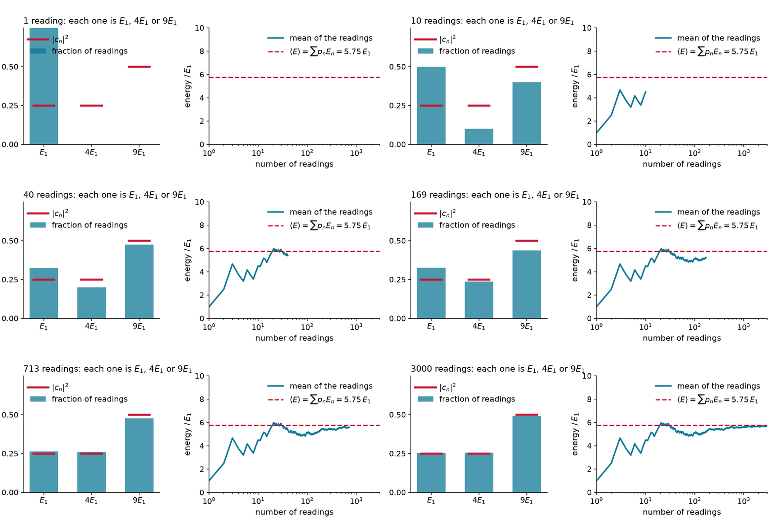
\text{reading } a_n \text{ with probability}\quad p_n = \lvert c_n\rvert^2 = \lvert\langle \phi_n \vert \psi \rangle\rvert^2

Live: measure it yourself

Averages and spreads

\langle A \rangle = \sum_n p_n\,a_n = \langle \psi \vert \hat{A} \vert \psi \rangle

\sigma_A^2 = \sum_n p_n\,\big(a_n - \langle A \rangle\big)^2 = \langle A^2 \rangle - \langle A \rangle^2

• \langle A\rangle: the average of many readings, usually not a possible reading itself
• \sigma_A = 0 only if all the probability sits on one eigenvalue: only eigenstates are sharp

Example: readings, average, spread

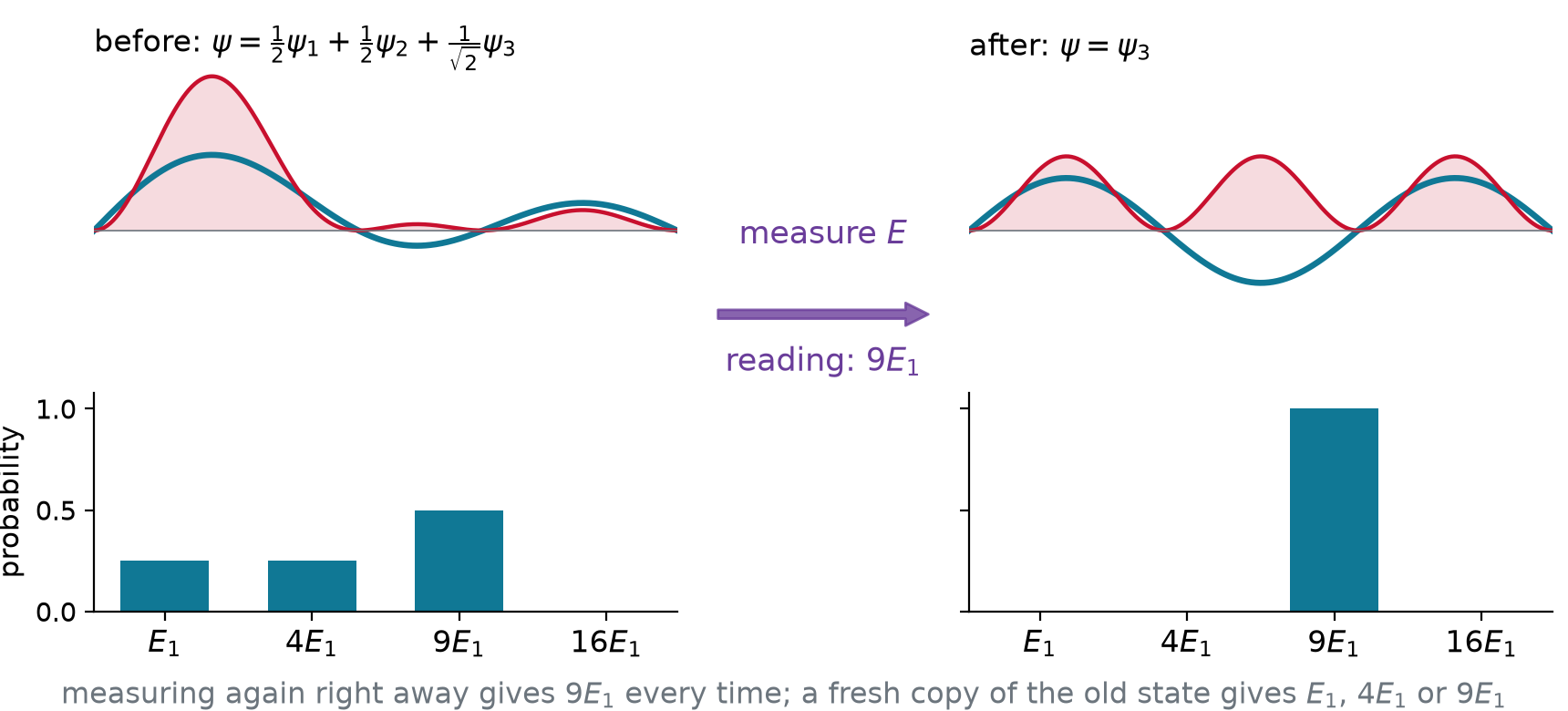
\psi = \tfrac{1}{2}\psi_1 + \tfrac{1}{2}\psi_2 + \tfrac{1}{\sqrt{2}}\psi_3 in a box. What can an energy measurement give, how often, and what are \langle E\rangle and \sigma_E?

E_1,\ 4E_1,\ 9E_1 \quad\text{with}\quad p = \tfrac{1}{4},\ \tfrac{1}{4},\ \tfrac{1}{2}

\langle E \rangle = \tfrac{1}{4}(1) + \tfrac{1}{4}(4) + \tfrac{1}{2}(9) = 5.75\,E_1

\langle E^2 \rangle = \tfrac{1}{4}(1) + \tfrac{1}{4}(16) + \tfrac{1}{2}(81) = 44.75\,E_1^2

\sigma_E = \sqrt{44.75 - 5.75^2}\;E_1 = 3.42\,E_1

After the measurement

• A reading of a_n leaves the state \phi_n (collapse): measure again, get a_n every time
• The probabilities live in many identical copies, not in one particle

A box state has no sharp momentum

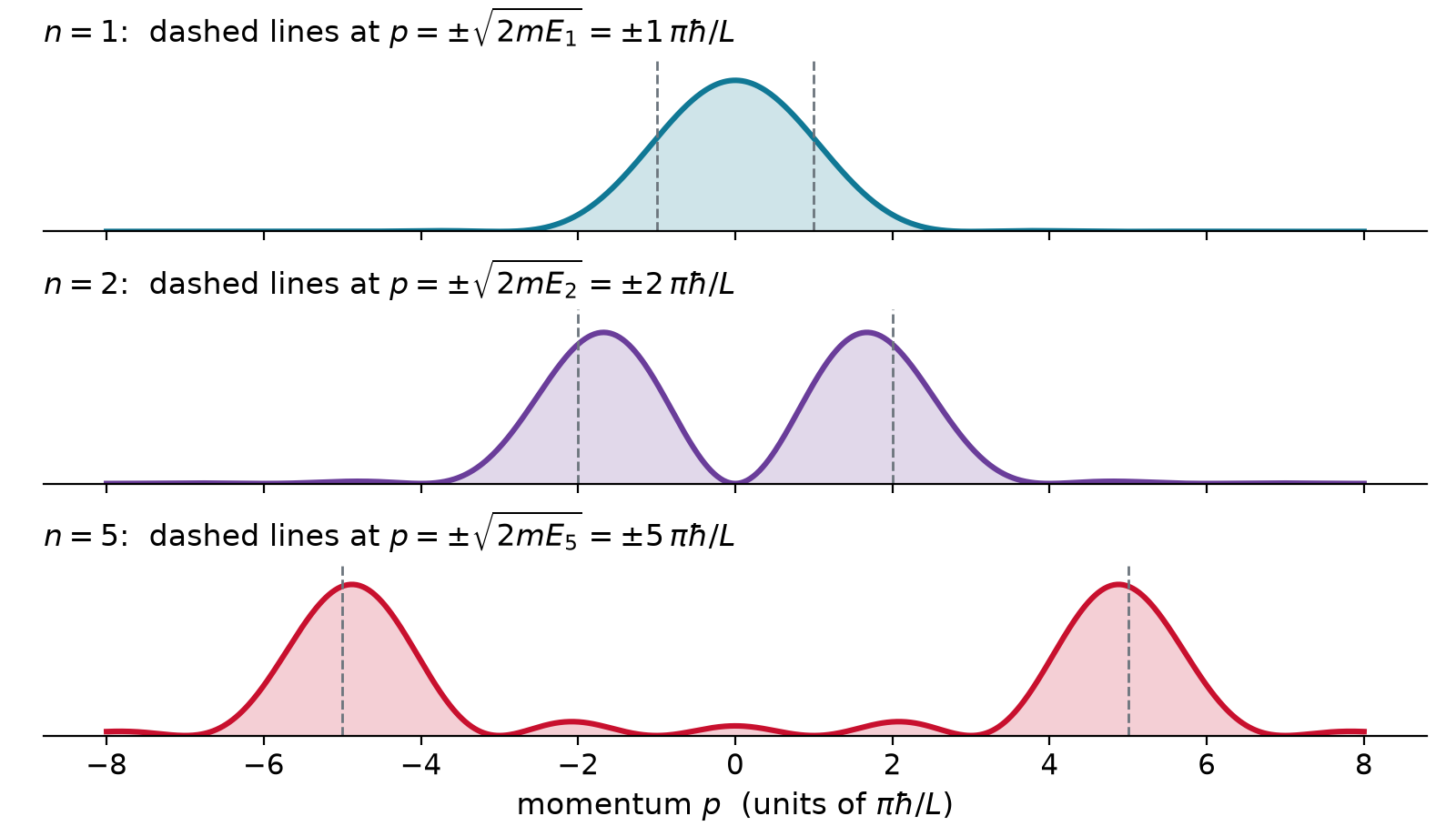
• \sin kx is half e^{ikx} (moving right), half e^{-ikx} (moving left); the walls broaden each hump
• Sharp E, spread p: in the box \hat{H} and \hat{p} do not share eigenfunctions

The uncertainty principle

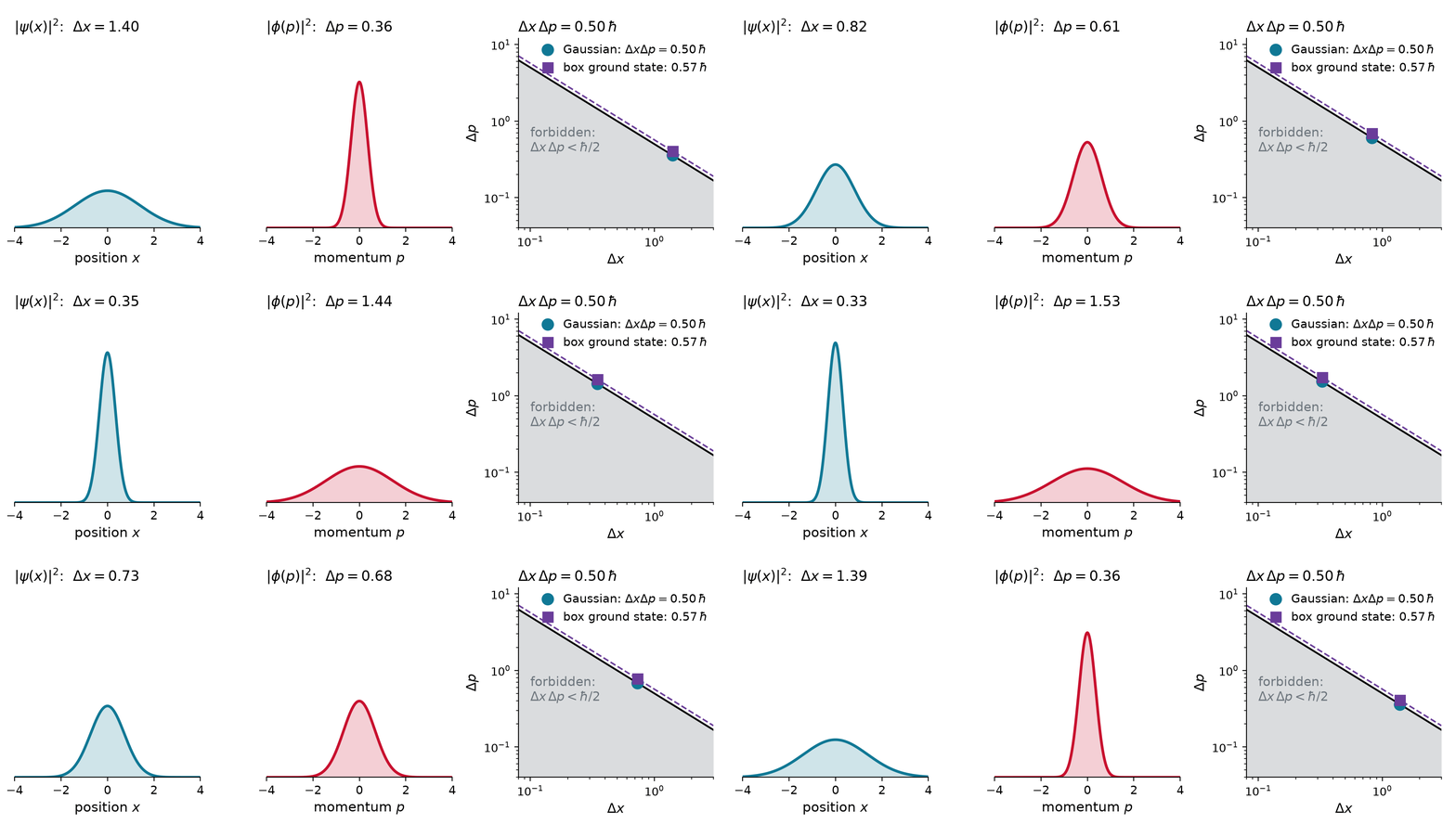
\sigma_A\,\sigma_B \geq \tfrac{1}{2}\big\lvert\langle[\hat{A},\hat{B}]\rangle\big\rvert \qquad\Longrightarrow\qquad \sigma_x\,\sigma_p \geq \hbar/2

Example: \sigma_x\sigma_p for the box ground state

For \psi_1 = \sqrt{2/L}\,\sin(\pi x/L), find \sigma_x, \sigma_p and their product.

\langle x\rangle = \tfrac{L}{2}, \quad \langle x^2\rangle = L^2\left(\tfrac{1}{3} - \tfrac{1}{2\pi^2}\right) \;\Rightarrow\; \sigma_x = 0.181\,L

\langle p\rangle = 0, \quad \langle p^2\rangle = 2mE_1 = \left(\tfrac{\pi\hbar}{L}\right)^2 \;\Rightarrow\; \sigma_p = \tfrac{\pi\hbar}{L}

\sigma_x\,\sigma_p = 0.181\,\pi\,\hbar = 0.568\,\hbar \;\geq\; 0.5\,\hbar

• Independent of L: squeeze the box and \sigma_p grows, so confinement costs energy (\propto 1/L^2)

Takeaway

Expand the state in the eigenfunctions of the observable: the coefficients are projections, c_n = \langle \phi_n \vert \psi \rangle. A measurement returns one eigenvalue a_n, with probability \lvert c_n\rvert^2, and leaves the system in \phi_n. Averages are weighted sums, \langle A\rangle = \sum_n \lvert c_n\rvert^2 a_n, sharp only in eigenstates; and observables that do not commute cannot be sharp together, \sigma_x\sigma_p \geq \hbar/2.