Time-Dependent Perturbation Theory and Selection Rules
Chem 3240 · Lecture 6.3
Why Time-Dependent Perturbations?
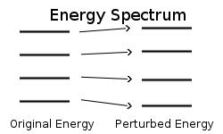
A time-dependent field can drive transitions between stationary states.
Light is an oscillating electromagnetic field.
This is the origin of spectroscopy and selection rules.
The Setup
- Split the Hamiltonian into a solvable part plus a weak, time-dependent kick.
\[\hat{H}(t) = \hat{H}_0 + \hat{V}(t), \qquad \hat{H}_0|n\rangle = E_n|n\rangle\]
- Expand the state in the stationary basis: \[|\Psi(t)\rangle = \sum_n c_n(t)\, e^{-iE_n t/\hbar}|n\rangle\]
- The coefficients \(c_n(t)\) carry all the dynamics.
Equation of Motion for the Coefficients
- Insert the expansion into the time-dependent Schrodinger equation.
\[i\hbar\,\dot{c}_m(t) = \sum_n c_n(t)\, V_{mn}(t)\, e^{i\omega_{mn}t}\]
\[V_{mn}(t) = \langle m|\hat{V}(t)|n\rangle, \qquad \omega_{mn} = \frac{E_m - E_n}{\hbar}\]
First-Order Transition Amplitude
- Start in state \(|i\rangle\). The perturbation is weak, so keep \(c_n \approx \delta_{ni}\).
\[\dot{c}_f^{(1)}(t) = -\frac{i}{\hbar}\, V_{fi}(t)\, e^{i\omega_{fi}t}\]
Integrate from \(0\) to \(t\): \[c_f^{(1)}(t) = -\frac{i}{\hbar}\int_0^t V_{fi}(t')\, e^{i\omega_{fi}t'}\, dt'\]
Coupling to Light: Dipole Approximation
- An oscillating field couples through the electric dipole.
\[\hat{V}(t) = -\hat{\boldsymbol{\mu}}\cdot\mathbf{E}(t), \qquad \mathbf{E}(t) = \mathbf{E}_0\cos(\omega t)\]
- Define the dipole matrix element \(\mu_{fi} = \langle f|\hat{\boldsymbol{\mu}}\cdot\hat{\mathbf{e}}|i\rangle\): \[V_{fi}(t) = -\mu_{fi}\, E_0\cos(\omega t)\]
Resonance and Energy Conservation
Write \(\cos(\omega t') = \tfrac{1}{2}(e^{i\omega t'} + e^{-i\omega t'})\).
The integral holds terms \(\displaystyle\int_0^t e^{i(\omega_{fi}\pm\omega)t'}\,dt'\).
Off-resonance these oscillate away. The amplitude is large only when \(\omega_{fi}\approx\omega\).
\[E_f - E_i = \pm\hbar\omega\]
Transition Probability
\[P_{i\to f}(t) \approx |c_f^{(1)}(t)|^2 \propto |\mu_{fi}|^2\]
The transition rate is set by the square of the dipole matrix element.
Allowed when \(\mu_{fi} = \langle f|\hat{\boldsymbol{\mu}}\cdot\hat{\mathbf{e}}|i\rangle \neq 0\).
Forbidden (first order) when symmetry makes it exactly zero.
Where Selection Rules Come From
A vanishing integral is dictated by symmetry, not by accident.
Wavefunctions: angular and parity symmetry of \(|i\rangle\) and \(|f\rangle\).
Operator: \(\hat{\boldsymbol{\mu}}\sim\mathbf{r}\) is a vector (angular-momentum-1) object.
The parity of the state must change for a dipole transition.
Selection Rules for Hydrogen-Like Atoms
- States are labeled \(|n, l, m_l\rangle\); \(\mathbf{r}\) transforms like \(Y_{1m}\).
Orbital angular momentum: \[\Delta l = l_f - l_i = \pm 1\]
Magnetic quantum number: \[\Delta m_l = m_{l,f} - m_{l,i} = 0, \pm 1\]
Takeaway
A weak oscillating field drives transitions with amplitude \(c_f^{(1)} = -\frac{i}{\hbar}\int_0^t V_{fi}\, e^{i\omega_{fi}t'}\,dt'\), large only at resonance \(E_f - E_i = \pm\hbar\omega\). The rate scales as \(|\mu_{fi}|^2\), and where symmetry makes this vanish the transition is forbidden: for hydrogen-like atoms \(\Delta l = \pm 1\), \(\Delta m_l = 0,\pm 1\).
Chem 3240 · Quantum Mechanics