Enhanced Sampling: Umbrella, Simulated Annealing, Parallel Tempering

Umbrella Sampling in the 2D Ising Model and Computation of $F(M)$ ¶

In the 2D Ising model, the magnetization $M = \sum_{i,j} s_{i,j}$ serves as a natural order parameter.
However, direct sampling of the full distribution of $M$ is often inefficient—particularly in systems near criticality or with metastable states—because rare magnetization states are seldom visited in unbiased simulations.
Umbrella sampling is a technique that improves sampling across the full magnetization range by adding a biasing potential that encourages the system to explore specified regions of phase space. Specifically, harmonic umbrella potentials of the form

U_{\text{bias}}(M) = \frac{1}{2} k (M - M_0)^2

(1)

These biased potentails are applied in separate simulations centered at different target magnetizations $M_0$ . This produces overlapping biased histograms of $M$ .

To recover the unbiased free energy profile $F(M)$ from these biased distributions, we apply either:

Histogram reweighting: Undo the bias using weights $\exp(\beta U_{\text{bias}})$ and stitch histograms together.
MBAR or WHAM: Statistically optimal reweighting of all biased samples to compute $F(M) = -k_B T \ln P(M)$ with uncertainty estimation.

The resulting $F(M)$ curve characterizes the thermodynamic landscape of the Ising model and reveals signatures of symmetry breaking, phase transitions, and metastability.

Biasing and recovering Free energies from simulations

:note, dropdown

In the canonical ensemble, the probability of observing a configuration $\{s_i\}$ of the 2D Ising model at temperature $T$ is:

P(\{s_i\}) = \frac{1}{Z} e^{-\beta E(\{s_i\})}

(2)

where:

$\beta = 1/(k_B T)$ ,
$E(\{s_i\})$ is the energy of the configuration,
$Z = \sum_{\{s_i\}} e^{-\beta E(\{s_i\})}$ is the partition function.

We are interested in the free energy as a function of magnetization:

M(\{s_i\}) = \sum_i s_i

(3)

The probability of observing a specific value of magnetization $M$ is given by:

P(M) = \frac{1}{Z} \sum_{\{s_i\}} \delta(M - M(\{s_i\})) e^{-\beta E(\{s_i\})}

(4)

and the associated free energy profile is:

F(M) = -k_B T \ln P(M) + \text{const}

(5)

However, in practice, directly sampling $P(M)$ is inefficient for rare values of $M$ . To overcome this, umbrella sampling introduces a bias potential $U_{\text{bias}}(M) = \frac{1}{2}k(M - M_0)^2$ and samples configurations from a biased ensemble:

P_{\text{bias}}(\{s_i\}; M_0) = \frac{1}{Z_{M_0}^{\text{bias}}} e^{-\beta \left[ E(\{s_i\}) + U_{\text{bias}}(M(\{s_i\})) \right]}

(6)

The biased partition function is:

Z_{M_0}^{\text{bias}} = \sum_{\{s_i\}} e^{-\beta \left[ E(\{s_i\}) + \frac{1}{2}k (M(\{s_i\}) - M_0)^2 \right]}

(7)

To recover the unbiased $P(M)$ , we reweight each sampled configuration from the biased ensemble:

P(M) \propto \left\langle \delta(M - M(\{s_i\})) \, e^{\beta U_{\text{bias}}(M(\{s_i\}))} \right\rangle_{\text{bias}}

(8)

This is performed across multiple overlapping biased ensembles with different centers $M_0$ , and the results are stitched together using methods such as:

Histogram reweighting, applying binning and weighted sums
WHAM (Weighted Histogram Analysis Method)
MBAR (Multistate Bennett Acceptance Ratio), which solves for the self-consistent probabilities of all sampled states

Finally, we obtain:

F(M) = -k_B T \ln P(M) + \text{const}

(9)

which captures the equilibrium free energy landscape as a function of magnetization — including phase coexistence and symmetry breaking near criticality.

import numpy as np
import matplotlib.pyplot as plt
from numba import njit

@njit
def total_energy(spins, J, B):
    """Total Ising energy with forward-bond counting (periodic BCs)."""
    N = spins.shape[0]
    E = 0.0
    for i in range(N):
        for j in range(N):
            S = spins[i, j]
            E -= J * S * (spins[(i + 1) % N, j] + spins[i, (j + 1) % N])
    E -= B * spins.sum()
    return E

@njit
def umbrella_run(spins, J, B, T, M0, k_bias,
                 n_equil, n_prod, out_freq):
    """Metropolis with a harmonic bias 0.5*k_bias*(M - M0)**2 on total M.

    Returns the final spins (to seed the next window) and the unbiased
    energies / total magnetizations sampled in the production phase.
    """
    N = spins.shape[0]
    E = total_energy(spins, J, B)
    M = spins.sum()

    n_samples = n_prod // out_freq
    E_out = np.empty(n_samples)
    M_out = np.empty(n_samples)
    k = 0

    for step in range(n_equil + n_prod):
        i = np.random.randint(N)
        j = np.random.randint(N)
        S = spins[i, j]
        nb = (spins[(i + 1) % N, j] + spins[(i - 1) % N, j]
              + spins[i, (j + 1) % N] + spins[i, (j - 1) % N])
        dE = 2.0 * S * (J * nb + B)
        M_new = M - 2 * S
        dU = 0.5 * k_bias * ((M_new - M0) ** 2 - (M - M0) ** 2)
        if (dE + dU) <= 0.0 or np.random.rand() < np.exp(-(dE + dU) / T):
            spins[i, j] = -S
            E += dE
            M = M_new

        if step >= n_equil and (step - n_equil) % out_freq == 0 and k < n_samples:
            E_out[k] = E
            M_out[k] = M
            k += 1

    return spins, E_out, M_out

# --- physical / numerical parameters --------------------------------------
N       = 20          # lattice side
T       = 2.0         # below Tc ≈ 2.269 so F(M) is double-welled
J, B    = 1.0, 0.0

# --- umbrella schedule ----------------------------------------------------
n_windows = 30
m_centers = np.linspace(-1.0, 1.0, n_windows)      # in units of m = M/N^2
M0_list   = m_centers * N**2                        # total-M centers used inside MC

# Window stiffness: sigma_M = sqrt(T/k) should be >= spacing between centers.
spacing_M = (M0_list[1] - M0_list[0])
k_bias    = 4.0 * T / spacing_M**2                  # sigma_M = spacing/2 -> ~95% overlap

# --- MC budget ------------------------------------------------------------
n_equil  = 50_000
n_prod   = 200_000
out_freq = 20

# --- run, seeding each window from the previous final config --------------
rng_seed = 0
np.random.seed(rng_seed)
spins = -np.ones((N, N), dtype=np.int64)            # start fully magnetized down

all_M, all_E = [], []
for M0 in M0_list:
    spins, E_out, M_out = umbrella_run(spins.copy(), J, B, T, M0, k_bias,
                                       n_equil, n_prod, out_freq)
    all_M.append(M_out)
    all_E.append(E_out)

all_M = [m.astype(float) for m in all_M]            # shape = n_windows x n_samples
print(f"k_bias = {k_bias:.4f}, samples/window = {len(all_M[0])}")

Diagnosing the biased histograms¶

A correct umbrella sampling run must satisfy two conditions:

Confinement. Each biased histogram is sharp around its target center $M_0$ .
Overlap. Adjacent histograms overlap so that every intermediate magnetization is visited by at least two windows.

We visualize the histograms in units of the magnetization per spin $m = M/N^2$ . If a window’s distribution drifts far from its center, it is undersampled (increase n_equil). If neighbors do not overlap, the windows are too far apart (add more centers or raise k_bias).

nbins   = 80
m_edges = np.linspace(-1.05, 1.05, nbins + 1)
m_grid  = 0.5 * (m_edges[1:] + m_edges[:-1])

fig, ax = plt.subplots(figsize=(9, 4))
for m0, Msamp in zip(m_centers, all_M):
    ax.hist(Msamp / N**2, bins=m_edges, density=True, alpha=0.4)
ax.set_xlabel(r'$m = M/N^2$')
ax.set_ylabel('biased density')
ax.set_title(f'Umbrella histograms ({n_windows} windows, $k={k_bias:.3f}$)')
ax.grid(True, ls=':', alpha=0.5)
plt.tight_layout()
plt.show()

Stitching the histograms: WHAM¶

The naive sum $\sum_k n_k(M)\,e^{+\beta U_k(M)}$ does not give $P(M)$ , because each biased ensemble has its own unknown normalization $Z_k^{\mathrm{bias}}$ . WHAM determines these constants self-consistently. Writing $f_k = Z_k^{\mathrm{bias}}/Z$ ,

P(M) \;=\; \frac{\sum_k n_k(M)}{\sum_k N_k\, f_k^{-1}\, e^{-\beta U_k(M)}},\qquad f_k \;=\; \sum_M P(M)\,e^{-\beta U_k(M)}\,\Delta M.

(10)

We iterate these two equations until the $f_k$ converge, then report $F(M) = -k_B T \ln P(M)$ .

def wham(all_M, M0_list, k_bias, beta, bin_edges,
         max_iter=2000, tol=1e-9):
    """Self-consistent binned WHAM on total-magnetization samples."""
    bin_centers = 0.5 * (bin_edges[1:] + bin_edges[:-1])
    bin_width   = np.diff(bin_edges)
    K           = len(all_M)

    # histograms and sample counts per window
    n_km = np.zeros((K, len(bin_centers)))
    N_k  = np.zeros(K)
    for k, M in enumerate(all_M):
        n_km[k], _ = np.histogram(M, bins=bin_edges)
        N_k[k]     = len(M)

    # bias evaluated at every bin center for every window
    U_km = 0.5 * k_bias * (bin_centers[None, :] - M0_list[:, None])**2
    w_km = np.exp(-beta * U_km)                    # Boltzmann weight

    numerator = n_km.sum(axis=0)                   # sum_k n_k(M)
    f_k       = np.ones(K)

    for it in range(max_iter):
        denom = (N_k[:, None] * w_km / f_k[:, None]).sum(axis=0)
        P     = np.zeros_like(denom)
        mask  = denom > 0
        P[mask] = numerator[mask] / denom[mask]
        norm  = (P * bin_width).sum()
        if norm <= 0:
            raise RuntimeError("WHAM: zero total probability; check sampling overlap.")
        P /= norm
        f_new = (P[None, :] * w_km * bin_width[None, :]).sum(axis=1)
        if np.max(np.abs(np.log(f_new / f_k))) < tol:
            f_k = f_new
            break
        f_k = f_new
    else:
        print(f"WHAM: reached max_iter={max_iter} without converging below {tol}")

    F = -np.log(np.where(P > 0, P, np.nan)) / beta
    F -= np.nanmin(F)
    return bin_centers, P, F, f_k

# --- run WHAM on the umbrella data ----------------------------------------
beta     = 1.0 / T
M_edges  = np.linspace(-1.05, 1.05, 101) * N**2
M_grid, P_M, F_M, f_k = wham(all_M, M0_list, k_bias, beta, M_edges)

# --- plot --------------------------------------------------------------------
fig, ax = plt.subplots(1, 2, figsize=(11, 4))

for Msamp in all_M:
    ax[0].hist(Msamp / N**2, bins=m_edges, density=True, alpha=0.35)
ax[0].plot(M_grid / N**2, P_M * N**2, 'k-', lw=2, label='WHAM $P(m)$')
ax[0].set_xlabel(r'$m$'); ax[0].set_ylabel('density')
ax[0].set_title('Biased histograms vs unbiased $P(m)$')
ax[0].legend(); ax[0].grid(True, ls=':', alpha=0.5)

ax[1].plot(M_grid / N**2, F_M, lw=2)
ax[1].set_xlabel(r'$m$'); ax[1].set_ylabel(r'$F(m)$')
ax[1].set_title(f'Free-energy profile at $T={T}$ (WHAM)')
ax[1].grid(True, ls=':', alpha=0.5)

plt.tight_layout()
plt.show()

Cross-check with MBAR (pymbar)¶

MBAR generalizes WHAM by reweighting individual samples rather than bins, yielding optimal estimates with analytical error bars. The key inputs are:

u_kn[k, n] — the reduced bias energy $\beta U_k(M_n)$ of sample $n$ evaluated under state $k$ . Every entry must be filled, not just the diagonal block.
u_n — the reduced potential of each sample in the target (unbiased) ensemble. Because the physical energy $\beta E$ is common to all windows (all at the same $T$ ), we can set u_n = 0: the constant cancels in MBAR.

!pip install pymbar

from pymbar import FES

# --- assemble sample array and per-window counts --------------------------
M_flat  = np.concatenate(all_M)                         # all total-M samples
N_k_arr = np.array([len(m) for m in all_M])
K       = len(M0_list)
Ntot    = len(M_flat)

# --- reduced potentials: fill EVERY (k, n) entry --------------------------
u_kn = np.empty((K, Ntot))
for k, M0 in enumerate(M0_list):
    u_kn[k, :] = beta * 0.5 * k_bias * (M_flat - M0)**2

# target (unbiased) reduced potential is zero — β E cancels across states
u_n = np.zeros(Ntot)

# --- FES via MBAR ---------------------------------------------------------
fes = FES(u_kn, N_k_arr, verbose=False)
fes.generate_fes(
    u_n=u_n,
    x_n=M_flat.reshape(-1, 1),
    fes_type='histogram',
    histogram_parameters={'bin_edges': [M_edges]},
)

query_pts = M_grid.reshape(-1, 1)
res       = fes.get_fes(query_pts, reference_point='from-lowest',
                        uncertainty_method='analytical')
F_mbar    = res['f_i'] / beta            # convert reduced -> physical units
dF_mbar   = res['df_i'] / beta

# --- compare WHAM vs MBAR --------------------------------------------------
fig, ax = plt.subplots(figsize=(7, 4))
ax.plot(M_grid / N**2, F_M, lw=2, label='WHAM')
ax.errorbar(M_grid / N**2, F_mbar, yerr=dF_mbar,
            fmt='o', ms=3, capsize=2, alpha=0.7, label='MBAR (pymbar)')
ax.set_xlabel(r'$m$'); ax.set_ylabel(r'$F(m)$')
ax.set_title(f'WHAM vs MBAR at $T={T}$')
ax.legend(); ax.grid(True, ls=':', alpha=0.5)
plt.tight_layout()
plt.show()

Sanity check: does umbrella sampling agree with brute force above $T_c$ ?¶

For $T > T_c$ the unbiased distribution is unimodal and easy to sample directly. If our umbrella + WHAM pipeline is correct, the reconstructed $F(m)$ must coincide with $-k_B T \ln P_{\mathrm{direct}}(m)$ obtained from a long plain-Metropolis run. Any systematic deviation points to insufficient equilibration, too-sparse windows, or a bug in the reweighting.

@njit
def plain_metropolis(spins, J, B, T, n_equil, n_prod, out_freq):
    N  = spins.shape[0]
    M  = spins.sum()
    n_samples = n_prod // out_freq
    M_out = np.empty(n_samples)
    k = 0
    for step in range(n_equil + n_prod):
        i = np.random.randint(N)
        j = np.random.randint(N)
        S = spins[i, j]
        nb = (spins[(i + 1) % N, j] + spins[(i - 1) % N, j]
              + spins[i, (j + 1) % N] + spins[i, (j - 1) % N])
        dE = 2.0 * S * (J * nb + B)
        if dE <= 0.0 or np.random.rand() < np.exp(-dE / T):
            spins[i, j] = -S
            M += -2 * S
        if step >= n_equil and (step - n_equil) % out_freq == 0 and k < n_samples:
            M_out[k] = M
            k += 1
    return M_out

T_hot   = 3.0
beta_h  = 1.0 / T_hot

# --- umbrella + WHAM at T_hot ---------------------------------------------
np.random.seed(1)
spins_h = np.ones((N, N), dtype=np.int64)
k_hot   = 4.0 * T_hot / spacing_M**2
all_M_h = []
for M0 in M0_list:
    spins_h, _, Msamp = umbrella_run(spins_h.copy(), J, B, T_hot, M0, k_hot,
                                     n_equil, n_prod, out_freq)
    all_M_h.append(Msamp)
_, _, F_umb, _ = wham(all_M_h, M0_list, k_hot, beta_h, M_edges)

# --- plain Metropolis reference at T_hot ----------------------------------
np.random.seed(2)
spins_p = np.ones((N, N), dtype=np.int64)
M_plain = plain_metropolis(spins_p, J, B, T_hot, n_equil, 2_000_000, out_freq)
P_plain, _ = np.histogram(M_plain, bins=M_edges, density=True)
F_plain    = -np.log(np.where(P_plain > 0, P_plain, np.nan)) / beta_h
F_plain   -= np.nanmin(F_plain)

fig, ax = plt.subplots(figsize=(7, 4))
ax.plot(M_grid / N**2, F_umb,   lw=2, label='umbrella + WHAM')
ax.plot(M_grid / N**2, F_plain, 'k--', lw=1.5, label='plain Metropolis')
ax.set_xlabel(r'$m$'); ax.set_ylabel(r'$F(m)$')
ax.set_title(f'Validation at $T={T_hot} > T_c$')
ax.set_ylim(bottom=-0.2)
ax.legend(); ax.grid(True, ls=':', alpha=0.5)
plt.tight_layout()
plt.show()

Simulated annealing¶

Is a widely used Monte Carlo technique used for numerical optimization In chemical and biological applications simulated annealing is used for finding global minima of a complex multidimensional energy functions>

Original paper: S. Kirkpatrick, C. D. Gelatt, Jr., M. P. Vecchi, Science 220, 671-680 (1983)

Simulated annealing in a nutshell¶

Introduce (artificial) temperature parameter $T$
Sample with metropolis algorithm where the acceptance probability takes the form $min (1, e^{-\Delta f/T})$
Here $f$ can be any function we want to minimize (not only energy)
For finding maximum simply change the sign: $min (1, e^{+\Delta f/T})$
Slowly reduce the temperature
“Slow cooling” is the main idea of simulated annealing

¶

very high $T$	very low $T$
almost all updates are accepted	only updates that decrease the energy are accepted
random configurations/explore entire space	descend towards minimum
high energy	low energy but might get stuck in local minimum

if we slowly cool from high $T$ to low $T$ we will explore the entire space until we converge to the (hopefully) global minimum
success is not guaranteed, but the methods works very well with good cooling schemes
Inspiration: annealing in metallurgy.
This is a great method to tackle NP-hard optimization problems, such as the traveling salesman!

Cooling schedules¶

slow cooling is essential: otherwise the system will “freeze” into a local minimum
but too slow cooling is inefficient...
initial temperature should be high enough so that the system is essentially random and equilibrates quickly
final temperature should be small enough so that we are essentially in the ground state (system no longer changes)
exponential cooling schedule is commonly used
$\boxed{T(t)=T_0e^{-t/\tau}}$
(11)
where $t$ is the Monte Carlo time and the constant $\tau$ needs to be determined (usually empirically)
alternative cooling schedules:
linear: $T(t)=T_0 - t/\tau$ (also widely used)
logarithmic: $T(t) = c/\log(1+t/\tau)$

Example: find global minimum of the function via simulated annealing: $f(x) = x^2 -\cos (4\pi x)$ ¶

f = lambda x: x*x - np.cos(4*np.pi*x) 
xvals = np.arange(-3,3,0.01)

plt.plot(xvals, f(xvals),lw=3)

plt.xlabel("$x$",fontsize=20)
plt.ylabel("$f(x)$",fontsize=20)
plt.grid(True)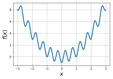

Search for global minima of $f(x)$ using simulated annealing¶

def MCupdate(T, x, mean=0.0, sigma=1.0):
    '''One Metropolis step: propose a Gaussian displacement, accept with
    Boltzmann probability at temperature T.'''
    xnew = x + np.random.normal(mean, sigma)
    delta_f = f(xnew) - f(x)
    if delta_f < 0 or np.random.rand() < np.exp(-delta_f / T):
        x = xnew
    return x

def cool(T, cool_t):
    '''Exponential cooling schedule: T(t) = T0 * exp(-t/tau).'''
    return T * np.exp(-1.0 / cool_t)

def sim_anneal(T=10, T_min=1e-4, cool_t=1e4, x=2, mean=0, sigma=1):
    
    '''Simulated annealing search for min of function:
    
    T=T0:        starting temperature
    T_min:       minimal temp reaching which sim should stop
    cool_t:      colling pace/time
    x=x0:        starting position 
    mean, sigma: parameters for diffusive exploration of x'''
    
    xlog   = []

    while T > T_min:
    
        x = MCupdate(T, x, mean, sigma)
    
        T = cool(T, cool_t)
   
        xlog.append(x)
    
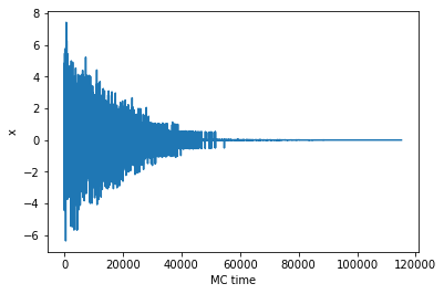
    return xlog

xlog = sim_anneal()

plt.plot(xlog)

plt.xlabel('MC time')
plt.ylabel('x')
print('Final search result for the global minimum: ', xlog[-1])

Final search result for the global minimum:  0.0012962682770579035

# Visualize descent: overlay annealed walker positions on the landscape
T0, x0, cool_t = 4.0, 2.0, 1e4
T, x = T0, x0
traj = [x]
for _ in range(3000):
    x = MCupdate(T, x, mean=0, sigma=1)
    T = cool(T, cool_t)
    traj.append(x)
traj = np.array(traj)

fig, ax = plt.subplots(figsize=(7, 4))
ax.plot(xvals, f(xvals), lw=2, color='steelblue', label='$f(x)$')
ax.scatter(traj, f(traj), c=np.arange(len(traj)), cmap='viridis', s=8, label='walker')
ax.set_xlim(-3, 3); ax.set_ylim(-1.5, 8)
ax.set_xlabel('$x$'); ax.set_ylabel('$f(x)$')
ax.set_title('Simulated annealing trajectory (color = time)')
ax.legend(); ax.grid(True, ls=':', alpha=0.5)
plt.tight_layout()

Challenges¶

Always slightly above the true minimum as long as $T>0$ .
Best combined with a local steepest-descent step at the end.

Simulated annealing applied to MCMC sampling of 2D Ising model¶

# Stub for Problem 2: simulated annealing on the 2D Ising model.
# Use the `mcmc` routine below as your inner sampler, and reduce T after
# each batch of sweeps according to the `cool` schedule. Record the lowest
# energy configuration seen.
temperature = 10.0    # initial temperature
tempmin     = 1e-4    # stop when T falls below this
cooltime    = 1e4     # cooling time tau for exponential schedule

def cool_schedule(T):
    return T * np.exp(-1.0 / cooltime)

Parallel tempering¶

Simulated annealing is not guaranteed to find the global extremum
- Unless you cool infinitely slowly.
- Usually need to repeat search multiple times using independent simulations.
Parallel tempering (aka Replica Exchange MCMC)
- Simulate several copies of the system in parallel
- Each copy is at a different constant temperature $T$
- Usual Metropolis updates for each copy
- Every certain number of steps attempt to exchange copies at neighboring temperatures
- Exchange acceptance probability is min(1, $e^{-\Delta f\Delta\beta}$ )
- If temperature difference small enough, the energy histograms of the copies will overlap and exhcanges will happen often.
Advantages of replica exchange:
- Exchanges allow to explore different extrema
- More successful for complex functions/energy landscapes. Random walk in temperature space!
- Detailed balance is maintained! (regular simulated annealing breaks detailed balance)

How to choose Temperature distributions for replica exchange MCMC¶

A dense temperature grid increases the exchange acceptance rates
But dense T grid takes longer to simulate and more steps are needed to move from one temperature to another
There are many options, often trial and error is needed
- exchange acceptance probability should be between about 20% and 80%
- exchange acceptance probability should be approximately temperature-independent
- commonly used: geometric progression for $N$ temperatures $T_n$ between and including $T_{\rm min}$ and $T_{\rm max}$ (ensures more steps around $T_{\rm min}$ )
  $T_n = T_{\rm min}\left(\frac{T_{\rm max}}{T_{\rm min}}\right)^{\frac{n-1}{N-1}}$
  (12)
make sure to spend enough time before swapping to achieve equilibrium!

parallel tempering simulation¶

# Parallel tempering for the 2D Ising model.
from numba import njit

@njit
def mcmc(spins, J, B, T, n_steps=10000, out_freq=1000):
    '''Metropolis sweep of a 2D Ising lattice at fixed (J, B, T).'''
    confs = []
    N = spins.shape[0]
    for step in range(n_steps):
        i = np.random.randint(N)
        j = np.random.randint(N)
        z = (spins[(i+1) % N, j] + spins[(i-1) % N, j]
             + spins[i, (j+1) % N] + spins[i, (j-1) % N])
        dE = 2 * spins[i, j] * (J * z + B)
        if dE <= 0 or np.random.rand() < np.exp(-dE / T):
            spins[i, j] *= -1
        if step % out_freq == 0:
            confs.append(spins.copy())
    return confs

@njit
def getE(spins, J, B):
    N = spins.shape[0]
    E = 0.0
    for i in range(N):
        for j in range(N):
            z = (spins[(i+1) % N, j] + spins[(i-1) % N, j]
                 + spins[i, (j+1) % N] + spins[i, (j-1) % N])
            E += -J * z * spins[i, j] / 4.0
    return E - B * spins.sum()

def temper(configs, T_list, J, B):
    '''Attempt to swap a random adjacent pair of replicas.'''
    i = np.random.randint(len(T_list) - 1)
    j = i + 1
    dBeta = 1.0 / T_list[i] - 1.0 / T_list[j]
    dE    = getE(configs[i][-1], J, B) - getE(configs[j][-1], J, B)
    if dBeta * dE < 0 or np.random.rand() < np.exp(-dBeta * dE):
        configs[i][-1], configs[j][-1] = configs[j][-1], configs[i][-1]
    return configs

def pt_mcmc(N, J, B, T_list, n_exch=1000, n_steps=10000, out_freq=1000):
    configs = [[np.random.choice(np.array([-1, 1]), size=(N, N)).astype(np.int64)]
               for _ in T_list]
    for _ in range(n_exch):
        configs = temper(configs, T_list, J, B)
        for k in range(len(T_list)):
            configs[k].extend(mcmc(configs[k][-1], J, B, T_list[k],
                                   n_steps=n_steps, out_freq=out_freq))
    return configs

%%capture
N = 20       # lattice side
J = 1.0      # coupling
B = 0.0      # external field

# Geometric ladder from T=1 (low, well-ordered) up through T_c=2.27 into disorder
T_list = np.geomspace(1.0, 5.0, 6)

n_exch = 200
configs = pt_mcmc(N, J, B, T_list, n_exch=n_exch, n_steps=2000, out_freq=200)

fig, ax = plt.subplots(figsize=(9, 4))
for k, Tk in enumerate(T_list):
    E = [getE(s, J, B) for s in configs[k]]
    ax.plot(E, lw=0.8, label=f'$T={Tk:.2f}$')
ax.set_xlabel('frame')
ax.set_ylabel('$E$')
ax.set_title('Replica energies along the parallel-tempering run')
ax.legend(fontsize=8, ncol=2)
ax.grid(True, ls=':', alpha=0.5)
plt.tight_layout()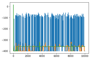

# Snapshots of the coldest replica (T = T_list[0]) across the run
snaps = configs[0]
idx = np.linspace(0, len(snaps) - 1, 6).astype(int)
fig, axes = plt.subplots(1, 6, figsize=(14, 2.5))
for ax, k in zip(axes, idx):
    ax.imshow(snaps[k], cmap='coolwarm', vmin=-1, vmax=1)
    ax.set_xticks([]); ax.set_yticks([])
    ax.set_title(f'frame {k}')
fig.suptitle(f'Coldest replica $T={T_list[0]:.2f}$', y=1.02)
plt.tight_layout()

Problems¶

Umbrella sampling. Use umbrella sampling to obtain the free-energy profile $F(M)$ below $T_c$ , at $T_c$ , and above $T_c$ (e.g. $T = 2.0, 2.269, 3.0$ ). Seed each window from the final configuration of the adjacent one to speed up equilibration.
Simulated annealing on the Ising model. Complete the stub in the simulated-annealing section below so that it finds the minimum-energy configuration of a 2D Ising model. Test with $B = 0$ (twofold degenerate ground state) and $B \neq 0$ (unique ground state).
Parallel tempering. Use parallel tempering to enhance sampling at $T = 1.0$ by coupling 8 replicas with $T > 1$ . Find the optimal $T$ spacing (target exchange-acceptance $\sim 30\%$ ) and compare histograms of the magnetization with a plain constant- $T$ Metropolis run.