Statistical Mechanics of Fluids

From phase space to the configurational integral¶

A classical fluid of $N$ particles in volume $V$ at temperature $T$ has a Hamiltonian that splits cleanly:

H(\mathbf{r}^N, \mathbf{p}^N) \;=\; \sum_{i=1}^N \frac{\mathbf{p}_i^{\,2}}{2m} \;+\; U(\mathbf{r}^N).

(1)

Because the kinetic and configurational pieces add, the canonical partition function factorizes:

Z(\beta, V, N) \;=\; \frac{1}{N!\, \lambda^{3N}} \underbrace{\int e^{-\beta U(\mathbf{r}^N)}\, d\mathbf{r}^N}_{\equiv\, Q(\beta, V, N)}, \qquad \lambda \;=\; \frac{h}{\sqrt{2\pi m k_B T}}.

(2)

The kinetic prefactor is exactly the ideal gas. Everything that makes a liquid a liquid lives in $Q$ , the configurational integral. Computing $Q$ analytically is impossible for any realistic $U$ — we need either approximations (mean-field theories, virial expansions) or simulations.

The pressure is

p \;=\; -\frac{\partial F}{\partial V} \;=\; k_B T \, \frac{\partial \ln Q}{\partial V}.

(3)

For a stable equilibrium fluid the volume dependence of $Q$ gives $p > 0$ , but a fluid stretched into the metastable region can sustain $p < 0$ transiently before cavitating — the inequality is a stability statement, not an absolute one.

Reduced distribution functions¶

We rarely need the full $N$ -body probability $P(\mathbf{r}^N) = e^{-\beta U}/Q$ . Most thermodynamic quantities depend only on low-order marginals. Define the $n$ -particle density

\rho^{(n)}(\mathbf{r}_1, \dots, \mathbf{r}_n) \;=\; \frac{N!}{(N-n)!} \int d\mathbf{r}_{n+1} \cdots d\mathbf{r}_N\, P(\mathbf{r}^N).

(4)

The combinatorial prefactor counts the $N!/(N-n)!$ ways to label particles at positions $\mathbf{r}_1, \dots, \mathbf{r}_n$ . For a homogeneous, isotropic fluid the one-body density is constant, $\rho^{(1)} = N/V \equiv \rho$ . The two-body density depends only on the separation $r = |\mathbf{r}_1 - \mathbf{r}_2|$ , and it defines the radial distribution function $g(r)$ via

\boxed{\;\rho^{(2)}(\mathbf{r}_1, \mathbf{r}_2) \;=\; \rho^{2}\, g(r)\;}

(5)

Read this as: $\rho\, g(r)$ is the local density at distance $r$ from a tagged particle. For an ideal gas $g(r) = 1$ everywhere; for a real fluid $g(r)$ is small at small $r$ (excluded volume), oscillates around 1 at intermediate $r$ (coordination shells), and approaches 1 at large $r$ (uncorrelated).

Reading $g(r)$ : shells, packing, structure¶

Three features of a liquid’s $g(r)$ encode different physics:

The first peak at $r \approx \sigma$ is the contact distance set by hard-core repulsion. Its height grows with density as the first solvation shell becomes more occupied.
The first minimum sets the boundary of the first coordination shell; integrating up to it gives the coordination number
$n_c \;=\; \rho \int_0^{r_{\min}} g(r)\, 4\pi r^2\, dr.$
(6)
Damped oscillations beyond the first peak reflect packing — like ripples around each particle. They die out at $r$ much larger than the correlation length.

The figures below contrast a dilute gas, dense gas, liquid, and crystal.

Hands-on: $g(r)$ from a 2D Lennard-Jones simulation¶

To make this concrete, run a quick Monte-Carlo simulation of a 2D Lennard-Jones fluid and measure $g(r)$ directly. The 2D normalization uses shell area $2\pi r\, dr$ instead of $4\pi r^2 dr$ :

g(r) \;=\; \frac{2 \,\langle n_{\text{pair}}(r) \rangle}{N \rho \cdot 2\pi r\, dr},

(7)

where $\langle n_{\text{pair}}(r) \rangle$ is the average histogram count of pair separations falling in the annulus $[r, r+dr]$ (each unordered pair counted once — hence the factor of 2).

import numpy as np
import matplotlib.pyplot as plt
from numba import njit

rng = np.random.default_rng(0)


@njit
def lj_mc_2d_with_gr(N, L, T, n_sweeps, max_disp, n_bins, r_max, seed):
    np.random.seed(seed)
    side = int(np.sqrt(N))
    pos = np.empty((N, 2))
    spacing = L / side
    for ix in range(side):
        for iy in range(side):
            k = ix * side + iy
            pos[k, 0] = (ix + 0.5) * spacing
            pos[k, 1] = (iy + 0.5) * spacing

    rcut2 = r_max * r_max
    hist = np.zeros(n_bins, dtype=np.int64)
    beta = 1.0 / T
    n_samples = 0

    for sweep in range(n_sweeps):
        for _ in range(N):
            i = np.random.randint(N)
            old_x, old_y = pos[i, 0], pos[i, 1]

            # energy of particle i at old position
            old_e = 0.0
            for j in range(N):
                if j == i:
                    continue
                dx = old_x - pos[j, 0]
                dy = old_y - pos[j, 1]
                dx -= L * round(dx / L)
                dy -= L * round(dy / L)
                r2 = dx * dx + dy * dy
                if r2 < rcut2 and r2 > 1e-12:
                    inv2 = 1.0 / r2
                    inv6 = inv2 * inv2 * inv2
                    old_e += 4.0 * (inv6 * inv6 - inv6)

            # propose move
            new_x = (old_x + (np.random.random() - 0.5) * 2.0 * max_disp) % L
            new_y = (old_y + (np.random.random() - 0.5) * 2.0 * max_disp) % L

            # energy at new position
            new_e = 0.0
            for j in range(N):
                if j == i:
                    continue
                dx = new_x - pos[j, 0]
                dy = new_y - pos[j, 1]
                dx -= L * round(dx / L)
                dy -= L * round(dy / L)
                r2 = dx * dx + dy * dy
                if r2 < rcut2 and r2 > 1e-12:
                    inv2 = 1.0 / r2
                    inv6 = inv2 * inv2 * inv2
                    new_e += 4.0 * (inv6 * inv6 - inv6)

            if np.random.random() < np.exp(-beta * (new_e - old_e)):
                pos[i, 0] = new_x
                pos[i, 1] = new_y

        # sample pair histogram after burn-in
        if sweep >= n_sweeps // 3:
            for i in range(N - 1):
                for j in range(i + 1, N):
                    dx = pos[i, 0] - pos[j, 0]
                    dy = pos[i, 1] - pos[j, 1]
                    dx -= L * round(dx / L)
                    dy -= L * round(dy / L)
                    r = np.sqrt(dx * dx + dy * dy)
                    if r < r_max:
                        b = int(r / r_max * n_bins)
                        if b < n_bins:
                            hist[b] += 1
            n_samples += 1

    return pos, hist, n_samples


def gr_from_hist(hist, n_samples, N, rho, r_max):
    n_bins = len(hist)
    edges = np.linspace(0, r_max, n_bins + 1)
    r = 0.5 * (edges[:-1] + edges[1:])
    dr = edges[1] - edges[0]
    shell = 2.0 * np.pi * r * dr                      # 2D shell area
    return r, 2.0 * hist / (n_samples * N * rho * shell)


# Run two densities at the same temperature
N, T, n_sweeps, max_disp, n_bins = 100, 1.5, 4000, 0.15, 80
results = {}
for rho in [0.3, 0.7]:
    L = np.sqrt(N / rho)
    _, hist, ns = lj_mc_2d_with_gr(N, L, T, n_sweeps, max_disp, n_bins, L / 2, 0)
    r, g = gr_from_hist(hist, ns, N, rho, L / 2)
    results[rho] = (r, g)

fig, ax = plt.subplots(figsize=(7, 4))
for rho, (r, g) in results.items():
    ax.plot(r, g, lw=1.5, label=fr'$\rho = {rho}$')
ax.axhline(1, color='k', lw=0.5)
ax.set(xlabel='$r$', ylabel='$g(r)$', xlim=(0, 4),
       title=f'2D Lennard-Jones $g(r)$ at $T={T}$')
ax.legend()
ax.grid(True, ls=':', alpha=0.5)
fig.tight_layout()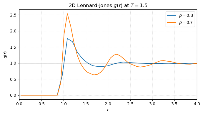

The dilute curve has only a small first peak; the dense curve develops the characteristic damped oscillations of a liquid. Both approach 1 at large $r$ — particles far away are uncorrelated.

The reversible work theorem: $g(r)$ as a free energy¶

There is a striking second reading of $g(r)$ . Define the potential of mean force $w(r)$ by

g(r) \;=\; e^{-\beta w(r)}, \qquad w(r) \;=\; -k_B T \ln g(r).

(8)

$w(r)$ is the reversible work required to bring two tagged particles from infinity to separation $r$ in the presence of all the others — fully equilibrated. Where $g(r)$ peaks, $w(r)$ has a minimum: a coordination-shell separation is favored. Where $g(r)$ dips below 1 (the trough between shells), $w(r)$ has a barrier.

This is more than a relabeling. The mean force at fixed separation is

\langle \mathbf{F}_{12}\rangle_r \;=\; -\nabla w(r) \;=\; k_B T\, \nabla \ln g(r),

(9)

so $w(r)$ governs the slow, large-scale motion of pairs of particles in a liquid — exactly the picture you need for diffusion, association, and reaction kinetics in solution.

# w(r) = -k_B T log g(r) from the simulated RDF
fig, ax = plt.subplots(figsize=(7, 4))
for rho, (r, g) in results.items():
    g_safe = np.where(g > 1e-3, g, 1e-3)
    w = -T * np.log(g_safe)
    ax.plot(r, w, lw=1.5, label=fr'$\rho = {rho}$')
ax.axhline(0, color='k', lw=0.5)
ax.set(xlabel='$r$', ylabel='$w(r) / k_B T$', xlim=(0.8, 4), ylim=(-1.2, 4),
       title='Potential of mean force')
ax.legend()
ax.grid(True, ls=':', alpha=0.5)
fig.tight_layout()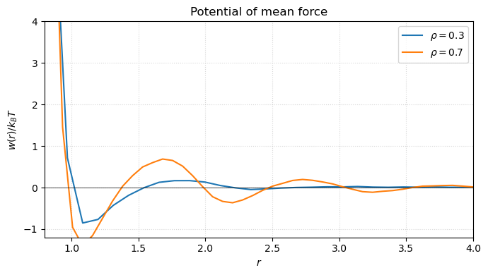

At low density $w(r)$ is essentially the bare LJ potential — $g(r) \to e^{-\beta u(r)}$ . At higher density correlations dress $w(r)$ : the well shifts, secondary minima appear, and the long-range tail picks up oscillatory structure. In water, for example, $w(r)$ between two methane-like solutes carries a desolvation barrier that is entirely a many-body effect.

Thermodynamics from $g(r)$ ¶

For pairwise interactions, $g(r)$ determines the most important fluid thermodynamic quantities. In 3D:

Energy per particle

\frac{\langle E\rangle}{N} \;=\; \frac{3}{2} k_B T \;+\; \frac{\rho}{2} \int_0^\infty g(r)\, u(r)\, 4\pi r^2\, dr.

(10)

Each particle has $\rho \cdot g(r) \cdot 4\pi r^2 dr$ neighbors at separation $r$ , each contributing $u(r)$ ; the factor of $1/2$ avoids double counting.

Pressure (virial equation)

\frac{p}{\rho k_B T} \;=\; 1 \;-\; \frac{\rho}{6 k_B T} \int_0^\infty r u'(r)\, g(r)\, 4\pi r^2\, dr.

(11)

The first term is the ideal gas; the integral is the virial correction. In an MD simulation $g(r)$ is what the histogram counts, and these two formulas turn it into thermodynamics.

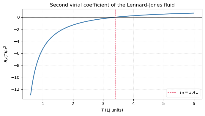
Low-density limit and the second virial coefficient¶

In the dilute limit, multi-body correlations are rare and a particle “feels” only its instantaneous partner:

g(r) \;\xrightarrow{\rho \to 0}\; e^{-\beta u(r)}.

(12)

Plug this into the pressure equation and Taylor-expand in $\rho$ to obtain the virial expansion

\frac{p}{k_B T} \;=\; \rho \;+\; B_2(T)\, \rho^2 \;+\; B_3(T)\, \rho^3 \;+\; \cdots,

(13)

where the second virial coefficient is

B_2(T) \;=\; -\frac{1}{2} \int_0^\infty \!\left[ e^{-\beta u(r)} - 1 \right] 4\pi r^2\, dr.

(14)

The integrand is the Mayer $f$ -function $f(r) = e^{-\beta u(r)} - 1$ . It captures deviations from ideality: $f(r) < 0$ in the repulsive core (excluded volume), $f(r) > 0$ in the attractive well (over-density).

At low $T$ attraction wins and $B_2 < 0$ — the gas attracts itself; at high $T$ excluded volume wins and $B_2 > 0$ , the gas repels itself.
The temperature where $B_2(T) = 0$ is the Boyle temperature $T_B$ , where the gas behaves ideally to second order despite microscopic interactions.

from scipy.integrate import quad
from scipy.optimize import brentq


def b2_lj(T, sigma=1.0, eps=1.0):
    '''B_2(T) for Lennard-Jones in 3D, in units of sigma^3.'''
    def integrand(r):
        u = 4.0 * eps * ((sigma / r) ** 12 - (sigma / r) ** 6)
        return (1.0 - np.exp(-u / T)) * r * r
    val, _ = quad(integrand, 1e-3, 8.0, limit=200)
    return 2.0 * np.pi * val


T_grid = np.linspace(0.6, 6.0, 120)
B2 = np.array([b2_lj(T) for T in T_grid])

T_Boyle = brentq(b2_lj, 2.0, 5.0)

fig, ax = plt.subplots(figsize=(7, 4))
ax.plot(T_grid, B2, color='steelblue', lw=2)
ax.axhline(0, color='k', lw=0.5)
ax.axvline(T_Boyle, color='crimson', ls='--', lw=1,
           label=fr'$T_B \approx {T_Boyle:.2f}$')
ax.set(xlabel='$T$ (LJ units)', ylabel=r'$B_2(T) / \sigma^3$',
       title='Second virial coefficient of the Lennard-Jones fluid')
ax.legend()
ax.grid(True, ls=':', alpha=0.5)
fig.tight_layout()

print(f'Boyle temperature for LJ: T_B = {T_Boyle:.4f}  (literature: ~3.418)')

Boyle temperature for LJ: T_B = 3.4083  (literature: ~3.418)

Takeaways¶

The whole fluid problem reduces to evaluating the configurational integral $Q$ , that is what simulation does.
$g(r)$ is the two-point marginal of the configurational distribution, and almost every thermodynamic quantity is a moment of $g(r)$ against some weight: energy weights it by $u(r)$ , pressure by $r u'(r)$ , virial coefficients by Mayer’s $f(r)$ .
$g(r)$ has a thermodynamic identity through the reversible-work theorem: $w(r) = -k_B T \ln g(r)$ is the free-energy profile felt by a pair embedded in the fluid.
The low-density expansion ( $g(r) \to e^{-\beta u}$ ) connects $B_2(T)$ directly to the pair potential and locates the Boyle temperature where attractive and repulsive contributions balance.

Problems¶

Coordination number. Run the 2D LJ simulation at $T = 1.5$ and $\rho = 0.7$ . Identify the location $r_{\min}$ of the first minimum of $g(r)$ and integrate $\rho \cdot g(r) \cdot 2\pi r\, dr$ from 0 to $r_{\min}$ — the result is the average number of first-shell neighbors. Repeat at $\rho = 0.3$ and $\rho = 0.85$ and report how the coordination number changes with density.
$B_2$ for the square-well potential. For $u(r) = +\infty$ for $r < \sigma$ , $-\varepsilon$ for $\sigma \le r < \lambda \sigma$ , and 0 for $r > \lambda \sigma$ , compute $B_2(T)$ analytically. Show that the Boyle temperature satisfies $\lambda^3 - 1 = (e^{\varepsilon/k_B T_B} - 1)^{-1}$ , i.e. $k_B T_B = \varepsilon / \ln(1 + 1/(\lambda^3 - 1))$ , and plot $T_B(\lambda)$ .
Pressure from $g(r)$ . From the simulated $g(r)$ at $\rho = 0.7$ , $T = 1.5$ compute the configurational contribution to the 2D pressure (replace $4\pi r^2$ with $2\pi r$ and $\frac{\rho}{6 k_B T}$ with $\frac{\rho}{4 k_B T}$ in the virial formula — the dimensional factors change). Compare to the ideal-gas value $\rho k_B T$ ; comment on its sign.

Reference¶

J.-P. Hansen and I. R. McDonald, Theory of Simple Liquids, 4th ed. (Academic Press, 2013) — chapters 2 (distribution functions) and 3 (perturbation theory). The standard text on everything above.

Statistical Mechanics of Fluids

From phase space to the configurational integral¶

Reduced distribution functions¶

Reading g(r)g(r)g(r): shells, packing, structure¶

Hands-on: g(r)g(r)g(r) from a 2D Lennard-Jones simulation¶

The reversible work theorem: g(r)g(r)g(r) as a free energy¶

Thermodynamics from g(r)g(r)g(r)¶