MFA applied to the Ising Model
In the Ising model, the mean-field approximation (MFA) decouples spin–spin interactions, reducing the system to a single macroscopic parameter: the average magnetization per spin, denoted by .
The factor of avoids double-counting spin pairs, and is the coordination number—for instance, for a 2D square lattice and for a 3D cubic lattice.
Derivation of the Mean-Field Hamiltonian
Consider the 2D Ising model where each spin interacts with its nearest neighbors:
Define the local mean field at site as:
Under the mean-field approximation, replace neighboring spins with their average value:
The total Hamiltonian then becomes:
Taking the thermal average and accounting for double counting leads to the previously derived mean-field expression for .
Self-Consistent Equation for Magnetization
Partition Function: After applying MFA, the system becomes effectively non-interacting, and the total partition function factorizes as , where is the partition function of a single spin. For :
The probability that a spin is in state is:
Average Magnetization: The mean value of a spin is then:
This self-consistent equation relates the average magnetization to itself via the hyperbolic tangent function, capturing the thermal competition between spin alignment and disorder.
Free Energy of Mean-Field Ising Models
Defining the Macrostate
Consider a spin lattice of sites, where each spin can point up or down. The total magnetization is given by:
Defining the magnetization per spin , the probabilities of spin-up and spin-down states are:
Entropy, Energy, and Free Energy
Entropy is given by the Shannon expression using the probabilities of spin states:
Energy in the mean-field approximation is the sum over spins in the presence of an average field:
Free Energy is the usual Legendre transform:
Dimensionless Free Energy per Spin (useful for analysis and plotting):
Source
import numpy as np
import matplotlib.pyplot as plt
from scipy.optimize import brentq
from matplotlib.animation import FuncAnimation
from IPython.display import HTML

# ---- shared MF Ising functions (J=1, q=4 so Tc = 4; we scale by Tc for clarity) ----
def f_ising(m, T_over_Tc):
    '''Dimensionless MF free energy per spin (in units of k_B T_c).'''
    eps = 1e-12
    m = np.clip(m, -1 + eps, 1 - eps)
    s = -((1 + m) / 2) * np.log((1 + m) / 2) - ((1 - m) / 2) * np.log((1 - m) / 2)
    e = -0.5 * m ** 2            # -Jq/2 m^2, with Jq = k_B T_c
    return e - T_over_Tc * s

m_grid = np.linspace(-1, 1, 400)
T_list = [0.6, 0.9, 1.0, 1.2, 1.5]
colors = plt.cm.viridis(np.linspace(0.15, 0.85, len(T_list)))

fig, ax = plt.subplots(figsize=(7, 4.5))
for T, c in zip(T_list, colors):
    f_vals = np.array([f_ising(m, T) for m in m_grid])
    ax.plot(m_grid, f_vals - f_vals.min(), color=c, lw=2,
            label=f'$T/T_c = {T:.1f}$')
ax.axvline(0, color='k', lw=0.5, alpha=0.4)
ax.set_xlabel('magnetization $m$')
ax.set_ylabel('$f(m) - f_{\\min}$   (shifted)')
ax.set_title('Mean-field free energy of the Ising model')
ax.legend()
ax.grid(True, ls=':', alpha=0.5)
plt.tight_layout()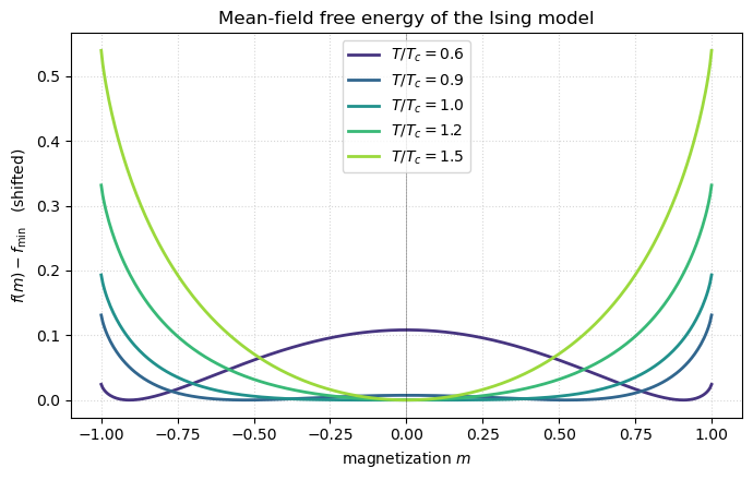
Visualizing the mean-field predictions
Three pictures tell the whole story of the mean-field Ising model:
The free energy as a function of magnetization at several temperatures: above it has a single minimum at ; below it has two minima at . That shape change is the phase transition.
The self-consistent equation solved graphically: a line intersects at the equilibrium magnetization.
The phase diagram : a two-dimensional map showing spontaneous magnetization below and its response to a field.
Finding the Critical Temperature
The critical point is determined by the second derivative of the free energy:
Magnetization as a Function of Temperature
The equilibrium magnetization minimizes the free energy, leading to a self-consistency condition:
Rearranged as:
For zero external field (), the equation simplifies to:
For small , expand , yielding:
Solving this, we find the magnetization near the critical point behaves as:
Below the curve develops two equal-depth minima at — spontaneous symmetry breaking. Above there is a single minimum at and the system is paramagnetic. Exactly at the curvature at vanishes: that is the mathematical fingerprint of a continuous phase transition.
Source
# Graphical solution of m = tanh((Tc/T) m)
fig, axes = plt.subplots(1, 3, figsize=(12, 3.8), sharey=True)
x = np.linspace(-2.5, 2.5, 400)
for ax, T in zip(axes, [0.7, 1.0, 1.4]):
    ax.plot(x, np.tanh(x), color='steelblue', lw=2, label=r'$\tanh(x)$')
    ax.plot(x, (T / 1.0) * x / 1.0, color='crimson', lw=2, ls='--',
            label=f'slope $T/T_c = {T}$')
    # find intersection numerically (positive branch)
    g = lambda xx: np.tanh(xx) - T * xx
    if g(0.1) * g(2.0) < 0:
        xroot = brentq(g, 0.1, 2.0)
        ax.scatter([xroot, -xroot, 0], [np.tanh(xroot), -np.tanh(xroot), 0],
                   color='k', zorder=5, s=45)
    else:
        ax.scatter([0], [0], color='k', zorder=5, s=45)
    ax.set_xlabel('$m$')
    ax.set_title(f'$T/T_c = {T}$')
    ax.grid(True, ls=':', alpha=0.5)
    ax.set_ylim(-1.3, 1.3)
    ax.legend(loc='lower right', fontsize=9)
axes[0].set_ylabel('value')
fig.suptitle('Self-consistency: intersection of $\\tanh(x)$ and $(T/T_c) x$', y=1.03)
plt.tight_layout()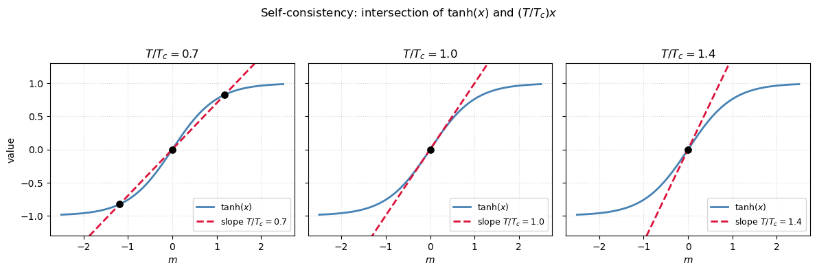
Source
import plotly.graph_objects as go
import numpy as np
from scipy.optimize import fsolve
from scipy.optimize import root_scalar  # Importing root_scalar

def compute_xcross(T, h_over_T):

    def f(M):
        Tc = 1.0  # Normalized temperature
        h = h_over_T * T  # Compute actual h from h/T and T
        return M - np.tanh((M + h) / (T / Tc))

    # Using symmetric interval for root finding to allow negative solutions
    interval = [-2.0, 2.0]

    # Check if a root is likely within the given range
    if f(interval[0]) * f(interval[1]) > 0:
        return 0.0  # If no root likely, return 0

    # Find the root using bisection method within the specified range
    result = root_scalar(f, bracket=interval, method='bisect')

    return result.root

# Define ranges for h/T  and T/Tc (from 0.2 to 1.5)
h_over_T_values = np.linspace(-0.2, 0.2, 101)
T_over_Tc_values = np.linspace(0.1, 1.6, 101)

# Create a meshgrid for T/Tc and h/T
H_over_T, T_over_Tc = np.meshgrid(h_over_T_values, T_over_Tc_values)

# Initialize an array for magnetizations
Magnetizations = np.zeros_like(H_over_T)

# Compute M for each (h/T, T/Tc) pair in the meshgrid
for i, T in enumerate(T_over_Tc_values):
    for j, h in enumerate(h_over_T_values):

        Magnetizations[i, j] = compute_xcross(T, h)


# Create a 3D surface plot using Plotly
fig = go.Figure(data=[go.Surface(z=Magnetizations, x=H_over_T, y=T_over_Tc,
                                 colorscale='RdBu',
                                 contours={
                                     #'z': {'show': True, 'start': -1.0, 'end': 1.0, 'size': 0.1, 'color':'orange'},
                                     'x': {'show': True, 'start': -1, 'end': 1, 'size': 0.05, 'color':'black'},
                                     'y': {'show': True, 'start': 0.5, 'end': 1.5, 'size': 0.1, 'color':'black'}
                                 })])

# Update plot layout
fig.update_layout(
    title='3D Plot of Magnetization M vs normalized temperature and field; T/Tc and h/T',
    scene=dict(
        xaxis_title='h/T',
        yaxis_title='T/Tc',
        zaxis_title='M',
        aspectmode='manual',
        yaxis_autorange='reversed',  # Reverse the Y-axis
        aspectratio=dict(x=2, y=2, z=0.75),  # Adjust these values as needed
        camera=dict(
            eye=dict(x=-4, y=-2, z=2),  # Adjust camera "eye" position for better view
            up=dict(x=0, y=0, z=1)  # Ensures Z is up
        )
    ),
    autosize=False,
    width=900,
    height=900
)

# Display the figure with configuration options
fig.show()Source
# Phase diagram m(h, T) computed by solving the self-consistency equation
def m_of_hT(h, T_over_Tc):
    '''Solve m = tanh(m/T_over_Tc + h/T_over_Tc).'''
    g = lambda m: m - np.tanh((m + h) / T_over_Tc)
    # Try a bracket that allows negative and positive roots
    try:
        return brentq(g, -1.0 + 1e-9, 1.0 - 1e-9)
    except ValueError:
        return np.nan

h_grid = np.linspace(-0.3, 0.3, 121)
T_grid = np.linspace(0.2, 1.6, 121)
H, Tm = np.meshgrid(h_grid, T_grid)
M = np.vectorize(m_of_hT)(H, Tm)

fig, ax = plt.subplots(figsize=(7.5, 5))
c = ax.pcolormesh(H, Tm, M, cmap='RdBu_r', vmin=-1, vmax=1, shading='auto')
ax.contour(H, Tm, M, levels=[-0.8, -0.4, 0, 0.4, 0.8],
           colors='k', linewidths=0.6, alpha=0.5)
ax.axhline(1.0, color='k', ls='--', lw=1)
ax.text(0.18, 1.03, '$T_c$', fontsize=11)
ax.set_xlabel('reduced field $h/J q$')
ax.set_ylabel('reduced temperature $T/T_c$')
ax.set_title('Phase diagram: magnetization $m(h, T)$')
fig.colorbar(c, ax=ax, label='$m$')
plt.tight_layout()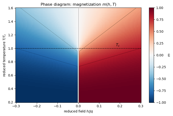
The dashed line at marks the critical isotherm. Below it the axis is a first-order line: the magnetization jumps discontinuously from to as crosses zero. Above it the crossover is smooth. The line terminates at the critical point — the end of the first-order line where the latent heat vanishes and the transition becomes continuous.
Landau theory: the universal form
Expanding the mean-field free energy around for ,
you get the Landau form
This is the universal skeleton of a continuous phase transition. The Ising model supplies the microscopic coefficients; the Landau expansion explains why very different systems — binary alloys, superconductors, liquid crystals, ferromagnets — share the same critical exponents. The only requirements are the symmetry of the order parameter and the analyticity of in it.
Source
# Landau free energy for positive, zero, negative quadratic coefficient
def f_landau(phi, a, b=1.0):
    return 0.5 * a * phi ** 2 + 0.25 * b * phi ** 4

phi = np.linspace(-2, 2, 400)
fig, ax = plt.subplots(figsize=(7, 4.2))
for a, label, color in zip(
        [1.0, 0.0, -1.0],
        ['$a > 0$ (disordered)', '$a = 0$ (critical)', '$a < 0$ (ordered)'],
        ['#1f77b4', '#ff7f0e', '#2ca02c']):
    ax.plot(phi, f_landau(phi, a), lw=2, label=label, color=color)
ax.axvline(0, color='k', ls='--', alpha=0.3)
ax.axhline(0, color='k', ls='--', alpha=0.3)
ax.set_xlabel(r'order parameter $\phi$')
ax.set_ylabel(r'$f(\phi)$')
ax.set_title('Landau free energy across the transition')
ax.legend()
ax.grid(True, ls=':', alpha=0.5)
plt.tight_layout()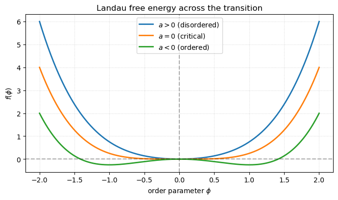
Dynamics of phase separation (Cahn–Hilliard)
Landau free energy plus a gradient penalty gives the Cahn–Hilliard equation
which conserves the total order parameter (the Laplacian outside ) and lets the system relax by interfacial motion rather than bulk nucleation. Starting from noise around with , the field rapidly separates into patches near the two Landau minima — the famous spinodal decomposition pattern.
Source
# Cahn-Hilliard simulation of spinodal decomposition on a periodic 2D grid
N = 128
dx = 1.0
dt = 0.01
steps = 1000
save_every = 10
epsilon = 1.0
a_land = -1.0
b_land = 1.0

def f_prime_land(phi):
    return a_land * phi + b_land * phi ** 3

def laplacian(field):
    return (
        -4 * field
        + np.roll(field, 1, axis=0) + np.roll(field, -1, axis=0)
        + np.roll(field, 1, axis=1) + np.roll(field, -1, axis=1)
    ) / dx ** 2

phi_field = 0.2 * np.random.rand(N, N) - 0.1
frames_ch = []
for step in range(steps):
    mu = -epsilon ** 2 * laplacian(phi_field) + f_prime_land(phi_field)
    phi_field += dt * laplacian(mu)
    if step % save_every == 0:
        frames_ch.append(phi_field.copy())

fig, ax = plt.subplots(figsize=(4.5, 4.5))
im = ax.imshow(frames_ch[0], cmap='bwr', vmin=-1, vmax=1)
ax.set_xticks([]); ax.set_yticks([])
title = ax.set_title('Cahn-Hilliard, $t = 0$')

def update_ch(k):
    im.set_array(frames_ch[k])
    title.set_text(f'Cahn-Hilliard, $t = {k * save_every * dt:.1f}$')
    return im, title

ani_ch = FuncAnimation(fig, update_ch, frames=len(frames_ch), interval=60, blit=False)
plt.close()
HTML(ani_ch.to_jshtml())Flory–Huggins: mean field for a binary mixture
The same mean-field logic that gave us the Ising transition also governs phase separation in mixtures — polymer solutions, oil/water demulsions, lipid rafts in membranes. The order parameter here is the volume fraction of one species (the other being ).
Place lattice sites; each site is either species (probability ) or (probability ). Two ingredients enter:
Entropy of mixing (Stirling on the number of arrangements):
Enthalpy of mixing (mean-field contact energy with one parameter that measures how much dislikes relative to and ):
The full Flory–Huggins free energy of mixing per site is therefore
Just like the MF Ising free energy, has a single minimum at high temperature (small ) and splits into two minima at low temperature (large ). The split happens at the critical point
which you can derive from . Because , the high- and low- phases are reversed compared to the Ising picture: large is the ordered (phase-separated) regime.
Why is Flory–Huggins a mean-field theory?
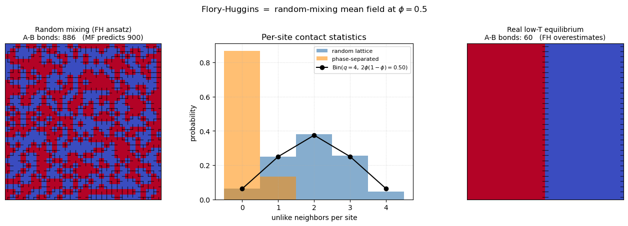
The derivation above secretly made one assumption: each lattice site is independently assigned species with probability or with probability , with no correlations between sites. Under this random-mixing ansatz a given lattice bond connects unlike species with probability
so the average contact energy per site is
which is precisely the term in . The figure below makes the assumption visible. Left: a lattice generated by independent Bernoulli draws at has the expected number of A–B bonds. Center: the per-site count of unlike neighbors follows a binomial — exactly as a textbook coin-flip problem would predict. Right: a real low-temperature equilibrium configuration at the same develops blobs of like species and has far fewer A–B contacts. Flory–Huggins treats every lattice as if it looked like the left panel. That is the mean-field step, and that is why the theory gets the coarse features of the phase diagram right but fails near , where those missing correlations dominate.
Source
# Why FH is a mean field: the "random mixing" assumption, made visible.
from scipy.stats import binom
import numpy as np
rng   = np.random.default_rng(1)
L     = 30
q     = 4            # square-lattice coordination number
phi   = 0.5          # equal-volume symmetric mixture

# (a) Random mixing = FH's hidden ansatz: every site is independent Bernoulli(phi)
lattice_random = (rng.random((L, L)) < phi).astype(np.int8)

# (b) Phase-separated reference at the SAME phi (shows what correlations look like)
lattice_split = np.zeros((L, L), dtype=np.int8)
lattice_split[:, :L // 2] = 1

def unlike_per_site(lat):
    """Number of opposite-species neighbors at each site (periodic BCs)."""
    return ((lat != np.roll(lat,  1, axis=0)).astype(int)
          + (lat != np.roll(lat, -1, axis=0)).astype(int)
          + (lat != np.roll(lat,  1, axis=1)).astype(int)
          + (lat != np.roll(lat, -1, axis=1)).astype(int))

def total_AB_bonds(lat):
    return int(((lat != np.roll(lat, 1, axis=0)).sum()
              + (lat != np.roll(lat, 1, axis=1)).sum()))

N_bonds   = 2 * L * L                          # 2 bonds per site (forward x, forward y)
p_opp     = 2 * phi * (1 - phi)                # FH's per-bond probability of A-B
MF_bonds  = p_opp * N_bonds                    # total A-B bonds predicted by FH
n_random  = total_AB_bonds(lattice_random)
n_split   = total_AB_bonds(lattice_split)

def draw_lattice(ax, lat, title):
    N_ = lat.shape[0]
    ax.imshow(lat, cmap='coolwarm', vmin=0, vmax=1)
    # overlay A-B bonds in black so the "contact energy" is visible
    for i in range(N_):
        for j in range(N_):
            if lat[i, j] != lat[(i + 1) % N_, j]:
                ax.plot([j, j], [i, i + 1], color='k', lw=0.9, alpha=0.7)
            if lat[i, j] != lat[i, (j + 1) % N_]:
                ax.plot([j, j + 1], [i, i], color='k', lw=0.9, alpha=0.7)
    ax.set_xlim(-0.5, N_ - 0.5); ax.set_ylim(N_ - 0.5, -0.5)
    ax.set_xticks([]); ax.set_yticks([])
    ax.set_title(title, fontsize=10)

fig, axes = plt.subplots(1, 3, figsize=(13.5, 4.4))

draw_lattice(axes[0], lattice_random,
             f'Random mixing (FH ansatz)\n'
             f'A-B bonds: {n_random}   (MF predicts {MF_bonds:.0f})')

c_rand  = unlike_per_site(lattice_random).ravel()
c_split = unlike_per_site(lattice_split).ravel()
bins    = np.arange(q + 2) - 0.5
xs      = np.arange(q + 1)

axes[1].hist(c_rand,  bins=bins, density=True, alpha=0.65,
             color='steelblue',  label='random lattice')
axes[1].hist(c_split, bins=bins, density=True, alpha=0.55,
             color='darkorange', label='phase-separated')
axes[1].plot(xs, binom.pmf(xs, q, p_opp), 'ko-', lw=1.5,
             label=fr'$\mathrm{{Bin}}(q{{=}}4,\,2\phi(1-\phi){{=}}{p_opp:.2f})$')
axes[1].set_xlabel('unlike neighbors per site')
axes[1].set_ylabel('probability')
axes[1].set_title('Per-site contact statistics')
axes[1].legend(fontsize=8, loc='upper right')
axes[1].grid(True, ls=':', alpha=0.5)

draw_lattice(axes[2], lattice_split,
             f'Real low-T equilibrium\n'
             f'A-B bonds: {n_split}   (FH overestimates)')

fig.suptitle(r'Flory-Huggins $= $ random-mixing mean field at $\phi = 0.5$',
             y=1.02, fontsize=12)
plt.tight_layout()
Source
# Flory-Huggins symmetric free energy (N_A = N_B = 1, per lattice site)
def f_FH(phi, chi):
    phi = np.clip(phi, 1e-12, 1 - 1e-12)
    return phi * np.log(phi) + (1 - phi) * np.log(1 - phi) + chi * phi * (1 - phi)

def fp_FH(phi, chi):
    return np.log(phi / (1 - phi)) + chi * (1 - 2 * phi)

def fpp_FH(phi, chi):
    return 1.0 / phi + 1.0 / (1 - phi) - 2 * chi

phi_grid = np.linspace(1e-3, 1 - 1e-3, 400)
chi_list = [1.5, 2.0, 2.3, 2.7, 3.2]
cmap = plt.cm.plasma(np.linspace(0.1, 0.85, len(chi_list)))

fig, ax = plt.subplots(figsize=(7.5, 4.5))
for chi, col in zip(chi_list, cmap):
    ax.plot(phi_grid, f_FH(phi_grid, chi), color=col, lw=2,
            label=f'$\\chi = {chi}$')
ax.axhline(0, color='k', lw=0.5, alpha=0.3)
ax.set_xlabel(r'volume fraction $\phi$')
ax.set_ylabel(r'$f(\phi)/k_B T$')
ax.set_title('Flory-Huggins free energy: single-well to double-well at $\\chi_c = 2$')
ax.legend()
ax.grid(True, ls=':', alpha=0.5)
plt.tight_layout()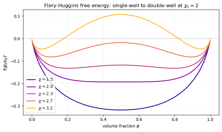
From to the phase diagram
At the free-energy curve has two minima and one maximum. To find the compositions that actually coexist in equilibrium we need the common-tangent construction: the two phases and that minimize the total free energy of a mixture of volume fractions lie on the same straight line tangent to . Equivalently,
For a symmetric mixture the construction degenerates to a horizontal tangent: by symmetry , and the two minima occur where . That curve is called the binodal — the boundary between a single homogeneous phase and two coexisting phases.
A second, inner curve comes from the spinodal, where the free energy loses convexity: . Between binodal and spinodal the homogeneous state is metastable — it is a local minimum and needs nucleation to decay. Inside the spinodal the homogeneous state is unstable and decays by spinodal decomposition, which is exactly what the Cahn–Hilliard animation above was showing.
Source
# Compute binodal and spinodal curves for the symmetric FH mixture
def binodal_phi(chi):
    '''Lower-phi minimum of f_FH (so phi < 0.5). Returns None below critical.'''
    if chi <= 2.0 + 1e-6:
        return None
    return brentq(lambda p: fp_FH(p, chi), 1e-6, 0.499)

def spinodal_phi(chi):
    if chi < 2.0:
        return None
    d = np.sqrt(1 - 2.0 / chi)
    return (1 - d) / 2.0

# Demonstrate common tangent for a specific chi > chi_c
chi_demo = 2.7
phi_b = binodal_phi(chi_demo)
phi_s = spinodal_phi(chi_demo)
tangent_y = f_FH(phi_b, chi_demo)   # horizontal tangent by symmetry

fig, ax = plt.subplots(figsize=(7.5, 4.5))
ax.plot(phi_grid, f_FH(phi_grid, chi_demo), color='steelblue', lw=2,
        label=f'$f(\\phi)$ at $\\chi = {chi_demo}$')
ax.axhline(tangent_y, color='crimson', ls='--', lw=1.5,
           label='common tangent')
ax.scatter([phi_b, 1 - phi_b], [tangent_y, tangent_y],
           color='crimson', s=70, zorder=5, label='binodal')
ax.scatter([phi_s, 1 - phi_s],
           [f_FH(phi_s, chi_demo), f_FH(1 - phi_s, chi_demo)],
           color='darkorange', marker='s', s=70, zorder=5, label='spinodal')
ax.axvspan(phi_b, phi_s, alpha=0.15, color='gray')
ax.axvspan(1 - phi_s, 1 - phi_b, alpha=0.15, color='gray',
           label='metastable')
ax.axvspan(phi_s, 1 - phi_s, alpha=0.25, color='darkorange',
           label='unstable (spinodal)')
ax.set_xlabel(r'$\phi$')
ax.set_ylabel(r'$f(\phi)/k_B T$')
ax.set_title(f'Common-tangent construction at $\\chi = {chi_demo}$')
ax.legend(loc='upper right', fontsize=9)
ax.grid(True, ls=':', alpha=0.5)
plt.tight_layout()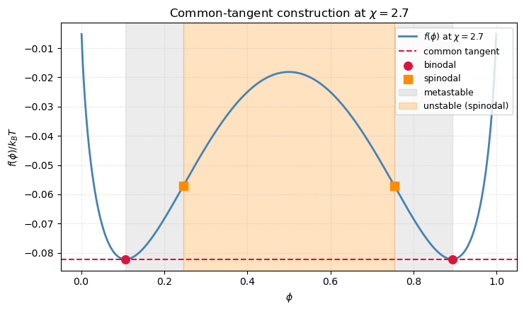
Source
# Full symmetric phase diagram in (phi, T/T_c) coordinates
# Since chi ~ 1/T, define T/T_c = chi_c/chi = 2/chi
chi_samples = np.linspace(2.001, 4.5, 200)
bino_left  = np.array([binodal_phi(c)  for c in chi_samples])
bino_right = 1 - bino_left
spin_left  = np.array([spinodal_phi(c) for c in chi_samples])
spin_right = 1 - spin_left
T_over_Tc = 2.0 / chi_samples

fig, ax = plt.subplots(figsize=(7.5, 5))
# Binodal (coexistence)
ax.plot(np.concatenate([bino_left, bino_right[::-1]]),
        np.concatenate([T_over_Tc, T_over_Tc[::-1]]),
        color='crimson', lw=2.5, label='binodal')
ax.fill(np.concatenate([bino_left, bino_right[::-1]]),
        np.concatenate([T_over_Tc, T_over_Tc[::-1]]),
        color='crimson', alpha=0.08)
# Spinodal (instability)
ax.plot(np.concatenate([spin_left, spin_right[::-1]]),
        np.concatenate([T_over_Tc, T_over_Tc[::-1]]),
        color='darkorange', lw=2, ls='--', label='spinodal')
ax.fill(np.concatenate([spin_left, spin_right[::-1]]),
        np.concatenate([T_over_Tc, T_over_Tc[::-1]]),
        color='darkorange', alpha=0.18)
# Critical point
ax.scatter([0.5], [1.0], color='k', s=80, zorder=6,
           label=r'critical point $(\phi_c, T_c)$')

ax.set_xlim(0, 1)
ax.set_ylim(T_over_Tc.min() * 0.95, 1.15)
ax.set_xlabel(r'volume fraction $\phi$')
ax.set_ylabel(r'$T / T_c \;=\; \chi_c / \chi$')
ax.set_title('Flory-Huggins phase diagram (symmetric mixture)')
ax.text(0.5, 1.08, 'mixed', ha='center', fontsize=10)
ax.text(0.5, 0.85, 'unstable\n(spinodal decomposition)',
        ha='center', fontsize=9, color='darkorange')
ax.text(0.17, 0.72, 'metastable', fontsize=9, color='crimson')
ax.text(0.83, 0.72, 'metastable', fontsize=9, color='crimson')
ax.legend(loc='lower center', fontsize=9)
ax.grid(True, ls=':', alpha=0.5)
plt.tight_layout()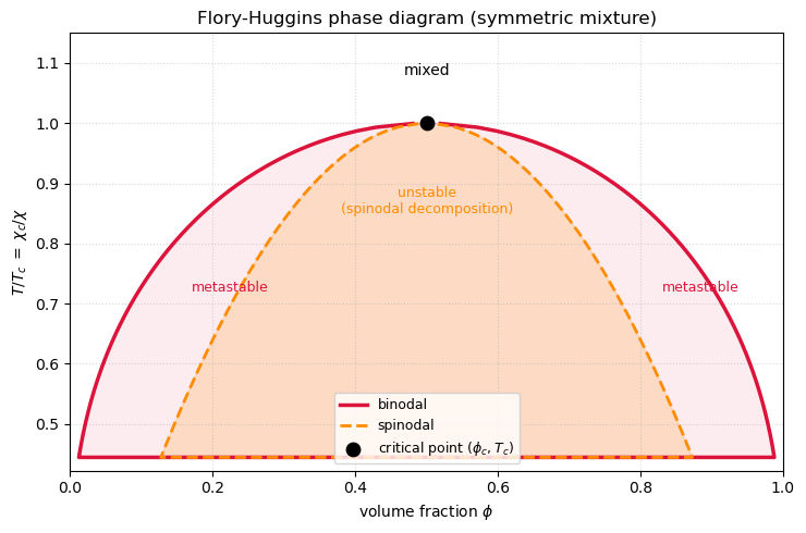
Sweeping : watching the phase diagram emerge
The animation below sweeps from 1.7 up to 3.5, corresponding to cooling from above the critical temperature into the two-phase region. The left panel redraws and the common-tangent / spinodal markers for the current . The right panel shows the full phase diagram with a moving horizontal slice at the current . As you cross the slice enters the miscibility gap and the free-energy curve opens up into a double well — the phase transition is literally drawn in front of you.
Source
# Animation: sweep chi from above Tc to well below
chi_frames = np.linspace(1.7, 3.5, 80)

# Precompute the static phase diagram curves (reuse from previous cell if available)
bino_vs_chi = []
spin_vs_chi = []
for c in chi_frames:
    bino_vs_chi.append(binodal_phi(c) if c > 2 else None)
    spin_vs_chi.append(spinodal_phi(c) if c >= 2 else None)

# Prebuild the phase diagram outline
chi_full = np.linspace(2.001, 4.5, 300)
bl = np.array([binodal_phi(c) for c in chi_full]); br = 1 - bl
sl = np.array([spinodal_phi(c) for c in chi_full]); sr = 1 - sl
TT = 2.0 / chi_full

phi_fine = np.linspace(1e-3, 1 - 1e-3, 300)

fig, axes = plt.subplots(1, 2, figsize=(12, 4.8))
line_f, = axes[0].plot([], [], color='steelblue', lw=2)
marker_bino = axes[0].scatter([], [], color='crimson', s=60, zorder=5, label='binodal')
marker_spin = axes[0].scatter([], [], color='darkorange', marker='s', s=60, zorder=5, label='spinodal')
tangent_line = axes[0].axhline(np.nan, color='crimson', ls='--', lw=1.2)
axes[0].set_xlim(0, 1)
axes[0].set_ylim(-0.8, 0.1)
axes[0].set_xlabel(r'$\phi$')
axes[0].set_ylabel(r'$f(\phi)/k_B T$')
axes[0].grid(True, ls=':', alpha=0.5)
axes[0].legend(loc='upper right', fontsize=9)
title_f = axes[0].set_title('')

axes[1].plot(np.concatenate([bl, br[::-1]]),
             np.concatenate([TT, TT[::-1]]),
             color='crimson', lw=2.3, label='binodal')
axes[1].plot(np.concatenate([sl, sr[::-1]]),
             np.concatenate([TT, TT[::-1]]),
             color='darkorange', lw=1.8, ls='--', label='spinodal')
axes[1].scatter([0.5], [1.0], color='k', s=60, zorder=5)
slice_line = axes[1].axhline(np.nan, color='steelblue', lw=2)
axes[1].set_xlim(0, 1)
axes[1].set_ylim(TT.min() * 0.95, 1.15)
axes[1].set_xlabel(r'$\phi$')
axes[1].set_ylabel(r'$T/T_c$')
axes[1].set_title('phase diagram')
axes[1].grid(True, ls=':', alpha=0.5)
axes[1].legend(loc='lower right', fontsize=9)

def update_fh(k):
    chi = chi_frames[k]
    Ttc = 2.0 / chi
    f_vals = f_FH(phi_fine, chi)
    line_f.set_data(phi_fine, f_vals)
    title_f.set_text(f'$\\chi = {chi:.2f}$   $T/T_c = {Ttc:.2f}$')
    pb = bino_vs_chi[k]
    ps = spin_vs_chi[k]
    if pb is not None:
        y = f_FH(pb, chi)
        marker_bino.set_offsets([[pb, y], [1 - pb, y]])
        tangent_line.set_ydata([y, y])
    else:
        marker_bino.set_offsets(np.empty((0, 2)))
        tangent_line.set_ydata([np.nan, np.nan])
    if ps is not None:
        marker_spin.set_offsets([[ps, f_FH(ps, chi)], [1 - ps, f_FH(1 - ps, chi)]])
    else:
        marker_spin.set_offsets(np.empty((0, 2)))
    slice_line.set_ydata([Ttc, Ttc])
    return line_f, marker_bino, marker_spin, tangent_line, slice_line

ani_fh = FuncAnimation(fig, update_fh, frames=len(chi_frames), interval=100, blit=False)
plt.close()
HTML(ani_fh.to_jshtml())Takeaways
Same recipe, different order parameters. MF Ising, Landau, and Flory–Huggins are all instances of the same procedure: write down a free energy as a function of a single macroscopic variable, minimize it, and watch the minimum structure change as a parameter crosses a critical value.
Universality is a feature, not a coincidence. Any symmetric analytic expanded around its critical point looks like . That is why alloys, magnets, and polymer solutions all share the same mean-field critical exponents (, , , ).
Binodal vs spinodal is the chemistry of real mixtures. Between them the system is metastable — it needs a nucleation event to phase separate. Inside the spinodal it is unstable and decomposes spontaneously, which is exactly the Cahn–Hilliard dynamics you saw.
Mean-field is quantitatively wrong but qualitatively everywhere. It fails near the critical point (wrong exponents) and for low dimensions (no transition in 1D), but it is the first-pass tool for any new phase-transition problem you will encounter.
Problems
Critical exponents from MF Ising. Using the mean-field self-consistency equation, show that near the magnetization scales as and the susceptibility as . Find and .
Asymmetric Flory–Huggins. Derive and plot the Flory–Huggins free energy of a polymer of length in a monomeric solvent,
Show that the critical point is and . Plot the binodal and spinodal for on the same axes and comment on the asymmetry.
Common tangent, the hard way. Modify the binodal code so it uses the general common-tangent equations (not the symmetry shortcut) and verify that it reproduces the same answer for the symmetric case. Then apply it to the asymmetric polymer case of Problem 2.
Cahn–Hilliard with Flory–Huggins. Replace the Landau in the Cahn–Hilliard cell with the Flory–Huggins derivative . Run at starting from and compare the morphology of the demixed pattern with the Landau version.
Lipid raft toy model. A cell membrane can be crudely modeled as a symmetric binary mixture of two lipid species with an effective that depends on temperature. Sketch the phase diagram, indicate where a cell at body temperature would sit, and argue whether you expect to see macroscopic phase separation or small metastable domains (“rafts”).