Surprise (self-information)
The sequences
have exactly the same probability for a fair coin:
So why does one feel shocking and the other boring?
How would you describe the sequence to a friend?
Frame problem in terms of micro and macro states.
A measure of information (whatever it may be) is closely related to the element of... surprise!
has very high probability and so conveys little information,
has very low probability and so conveys much information.
If we quanitfy suprise we will quantify information
Addititivity of Information
Knowledge leads to gaining information
Which is more surprising (contains more information)?
E1: The card is heart?
E2:The card is Queen?
E3: The card is Queen of hearts?
Knowledge of event should add up our information:
We learn the card is heart
We learn the card is Queen
A logarithm of probability is a good candidate function for information!
What about the sign?
This quantifies surprise or self-information associated with one specific event or microstate with probability
Why bit (base two)
Consider symmetric a 1D random walk with equal jump probabilities. We can view Random walk = string of Yes/No questions.
Imagine driving to a location how many left/right turn informations you need to reach destination?
You gain one bit of information when you are told Yes/No answer
To decode N step random walk trajectory we need N bits.
Shannon Entropy and Information
If we want to understand the overall uncertainty in the system, we need to consider all possible outcomes weighted by their probability of occurrence.
This means that rather than looking at the surprise of a single event, we consider the average surprise one would experience over many trials drawn from .
Thus, we take the expectation of surprise over the entire distribution arriving at a formula known as Shaonon’s expression of Entropy.
One often uses to denote Shanon Entropy () and letter with for entropy in units of Boltzman constant
For now lets just roll with we wont be doing any thermodynamics in here.
John von Neumann advice to [To Calude Shanon], "You should call it Entropy, for two reasons. In the first place you uncertainty function has been used in statistical mechanics under that name. In the second place, and more importantly, no one knows what entropy really is, so in a debate you will always have the advantage.”
Source
import numpy as np
import matplotlib.pyplot as plt

def binary_entropy(p):
    """
    Compute the binary Shannon entropy for a given probability p.
    Avoid issues with log(0) by ensuring p is never 0 or 1.
    """
    return -p * np.log2(p) - (1 - p) * np.log2(1 - p)

# Generate probability values, avoiding the endpoints to prevent log(0)
p_vals = np.linspace(0.001, 0.999, 1000)
H_vals = binary_entropy(p_vals)

# Create a figure with two subplots side-by-side
fig, ax = plt.subplots(1, 2, figsize=(14, 6))

# Plot 1: Binary Shannon Entropy Function
ax[0].plot(p_vals, H_vals, lw=4, color='midnightblue',
           label=r"$H(p)=-p\log_2(p)-(1-p)\log_2(1-p)$")
ax[0].set_xlabel(r"Probability $p$)", fontsize=14)
ax[0].set_ylabel("Entropy (bits)", fontsize=14)
ax[0].set_title("Binary Shannon Entropy",  fontsize=16)
ax[0].legend(fontsize=12)
ax[0].grid(True)

# Plot 2: Example Distributions and Their Entropy
# Define a few example two-outcome distributions:
distributions = {
    "Uniform (0.5, 0.5)": [0.5, 0.5],
    "Skewed (0.8, 0.2)": [0.8, 0.2],
    "Extreme (0.99, 0.01)": [0.99, 0.01]
}

# Colors for each distribution
colors = ["skyblue", "salmon", "lightgreen"]

# For visual separation, use offsets for the bars
width = 0.25
x_ticks = np.arange(2)  # positions for the two outcomes

for i, (label, probs) in enumerate(distributions.items()):
    # Compute the Shannon entropy for the distribution
    entropy_val = -np.sum(np.array(probs) * np.log2(probs))
    # Offset x positions for clarity
    x_positions = x_ticks + i * width - width
    ax[1].bar(x_positions, probs, width=width, color=colors[i],
              label=f"{label}\nEntropy = {entropy_val:.2f} bits")

# Set labels and title for the bar plot
ax[1].set_xticks(x_ticks)
ax[1].set_xticklabels(["Outcome 1", "Outcome 2"], fontsize=12)
ax[1].set_ylabel("Probability", fontsize=14)
ax[1].set_title("Example Distributions", fontsize=16)
ax[1].legend(fontsize=12)
ax[1].grid(True, axis='y')

plt.tight_layout()
plt.show()
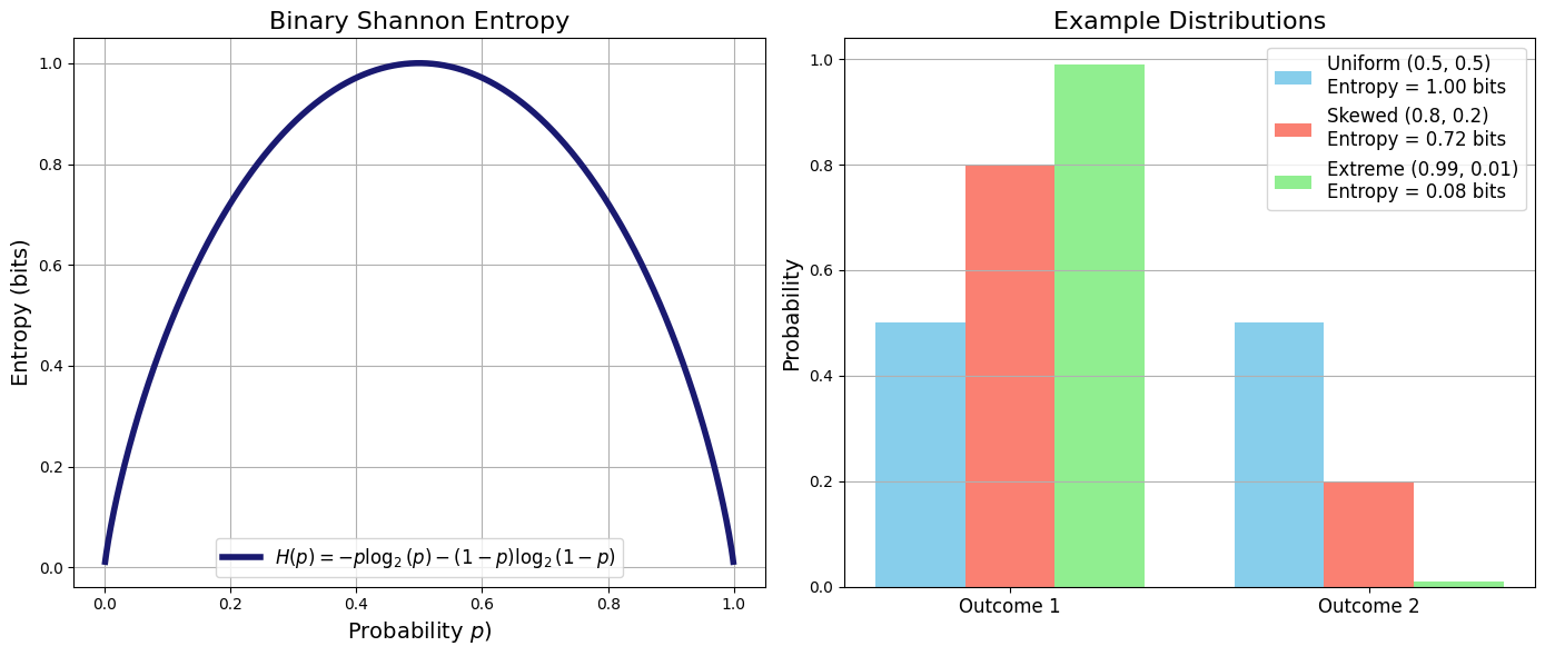
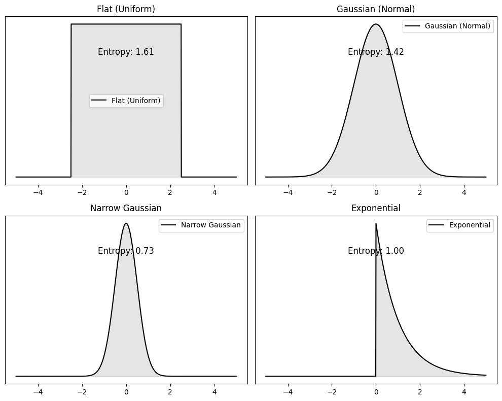
To reiterate once again from Shannon formula we see clearly that Entropy is a statistical quantity characterized by the probability distribution over all possibilities.
The more uncertain (unpredictable) the outcome the higher the entropy of the probability distribution that generates it.
Source
import numpy as np
import scipy.stats as stats
import matplotlib


# Create figure and axes
fig, axes = plt.subplots(2, 2, figsize=(10, 8))

# Define x range
x = np.linspace(-5, 5, 1000)

# Define different distributions
distributions = {
    "Flat (Uniform)": stats.uniform(loc=-2.5, scale=5),
    "Gaussian (Normal)": stats.norm(loc=0, scale=1),
    "Narrow Gaussian": stats.norm(loc=0, scale=0.5),
    "Exponential": stats.expon(scale=1)
}

# Plot distributions and annotate entropy
for ax, (name, dist) in zip(axes.flatten(), distributions.items()):
    pdf = dist.pdf(x)
    ax.plot(x, pdf, label=name, color='black')
    ax.fill_between(x, pdf, alpha=0.2, color='gray')

    # Compute differential entropy
    entropy = dist.entropy()
    ax.text(0, max(pdf) * 0.8, f"Entropy: {entropy:.2f}", fontsize=12, ha='center')

    ax.set_title(name)
    ax.set_yticks([])
    ax.legend()

# Adjust layout and show plot
plt.tight_layout()
plt.show()
Exercise: Information per letter to decode the message
Let represent the letters in an alphabet. For example:
Korean: 24 letters
English: 26 letters
Russian: 33 letters
The information content associated with these alphabets satisfies:
The information of a sequence of letters is additive, regardless of the order in which they are transmitted:
Question If the symbols of English alphabet (+ blank) appear equally probably, what is the information carried by a single symbol? This must be bits, but for actual English sentences, it is known to be about 1.3 bits. Why?
Solution
Not every letter has equal probability or frequency of appearing in a sentence!
Exercise: entropy of die rolls
How much knowledge we need to find out outcome of fair dice?
We are told die shows a digit higher than 2 (3, 4, 5 or 6). How much knowledge does this information carry?
Solution
Exercise: Monty Hall problem
There are five boxes, of which one contains a prize. A game participant is asked to choose one box. After they choose one of the five boxes, the “coordinator” of the game identifies as empty three of the four unchosen boxes. What is the information of this message?
Solution
Exercise: Why are there non-integer number of YES/NO questions??
Explain the origin of the non-integer information. Why it takes less than one-bit to encode information?
Solution
We have encountered a fraction of bit of information several times now. What does it imply in terms of number of YES/NO questions. That is becasue in some cases single YES/NO question can rule out more than one elementary event.
In other words we can ask clever questions that can get us to answer faster than doing YES/No on every single possibility
999 blue balls and 1 red ball. how many questions we need to ask to determin the colors of all balls? bit or 0.01 bit per ball. Divide the container by 500 and 500 and ask where the red ball is? 1 questions rules out 500 balls at once.
Entropy, micro and macro states
When all number of microstates of the system have equal probability the entropy of the system is:
We arrive at an expression of Entropy first obtained by Boltzmann where thermal energy units (Boltzman’s) constant were used.
Entropy for a macrostate A which has number of microstates can be written in terms of macrostate probability
Entropy of a macrostate quantifies how probable that macrostate is!. This is yet another manifestation of Large Deviation Theorem we encountered before
Flashback to Random Walk, Binomial, and Large Deviation Theorem
Probability of a macrostate of (n gas particles out of N landing in right hand side of container):
where is the total number of microstates.
When we took the log of this we called it entropy but why?
Here, represents the fraction (empirical probability) of steps to the right in a random walk.
is the entropy per particle (or per step), while is the total entropy.
Connection to the Large Deviation Theorem
When we express probability in terms of entropy, we recover the Large Deviation Theorem, which states that fluctuations from the most likely macrostates are exponentially suppressed:
This result highlights how entropy naturally governs the likelihood of macrostates in statistical mechanics.
Source
import numpy as np
import matplotlib.pyplot as plt
from matplotlib.animation import FuncAnimation
from IPython.display import HTML, display

# Render inline (web) as HTML/JS
plt.rcParams["animation.html"] = "jshtml"

# -----------------------------
# Gas-in-a-box animation (2D) + live macrostate histogram
# -----------------------------
rng = np.random.default_rng(0)

# Box
W, H = 1.0, 1.0
divider_x = W / 2

# Particles + dynamics
N = 400
dt = 0.01
speed = 0.55          # increase for faster motion
frames = 900
interval_ms = 30

# Initialize particles (start mostly on LEFT to show mixing)
x = rng.random(N) * (0.45 * W)
y = rng.random(N) * H

theta = rng.random(N) * 2 * np.pi
vx = speed * np.cos(theta)
vy = speed * np.sin(theta)

# Macrostate tracking: nL(t)
nL_history = []
maxN = N
# histogram bins for nL = 0..N
bin_edges = np.arange(-0.5, N + 1.5, 1.0)
centers = np.arange(0, N + 1)

# -----------------------------
# Figure
# -----------------------------
fig = plt.figure(figsize=(10, 4.2))
gs = fig.add_gridspec(1, 2, width_ratios=[1.1, 1.4])

ax_box = fig.add_subplot(gs[0, 0])
ax_hist = fig.add_subplot(gs[0, 1])

# Box plot
ax_box.set_title("2D gas in a box")
ax_box.set_xlim(0, W)
ax_box.set_ylim(0, H)
ax_box.set_aspect("equal", adjustable="box")
ax_box.axvline(divider_x, lw=2)
ax_box.set_xticks([])
ax_box.set_yticks([])

scat = ax_box.scatter(x, y, s=10)
txt_box = ax_box.text(0.02, 1.02, "", transform=ax_box.transAxes, va="bottom")

# Histogram plot
ax_hist.set_title(r"Histogram of $n_L$ over time (macrostate occupancy)")
ax_hist.set_xlabel(r"$n_L$")
ax_hist.set_ylabel("count")

counts0 = np.zeros_like(centers, dtype=int)
bars = ax_hist.bar(centers, counts0, width=0.9, align="center")
ax_hist.set_xlim(-1, N + 1)
ax_hist.set_ylim(0, 10)

txt_hist = ax_hist.text(0.02, 0.98, "", transform=ax_hist.transAxes, va="top")

# -----------------------------
# Helper: Shannon entropy of the *empirical* macrostate distribution P(nL)
# -----------------------------
def shannon_entropy_from_counts(counts):
    total = counts.sum()
    if total == 0:
        return 0.0
    p = counts[counts > 0] / total
    return float(-(p * np.log(p)).sum())

# -----------------------------
# Animation update
# -----------------------------
def update(frame):
    global x, y, vx, vy

    # Free-flight
    x = x + vx * dt
    y = y + vy * dt

    # Reflect at walls (elastic)
    hit_left = x < 0
    hit_right = x > W
    vx[hit_left | hit_right] *= -1
    x = np.clip(x, 0, W)

    hit_bottom = y < 0
    hit_top = y > H
    vy[hit_bottom | hit_top] *= -1
    y = np.clip(y, 0, H)

    # Update scatter
    scat.set_offsets(np.column_stack([x, y]))

    # Macrostate: how many on left?
    nL = int(np.sum(x < divider_x))
    nR = N - nL
    nL_history.append(nL)

    # Histogram of nL over time
    hist_counts, _ = np.histogram(nL_history, bins=bin_edges)
    for b, h in zip(bars, hist_counts):
        b.set_height(h)

    # Autoscale histogram y
    ymax = max(10, int(hist_counts.max()) + 2)
    if ax_hist.get_ylim()[1] < ymax:
        ax_hist.set_ylim(0, ymax)

    # Compute "entropy" of macrostate occupancy (empirical Shannon entropy)
    S = shannon_entropy_from_counts(hist_counts)

    txt_box = ax_box.text(
    0.02, 0.96,
    "",
    transform=ax_box.transAxes,
    va="top",
    fontsize=10,
    bbox=dict(facecolor="white", alpha=0.7, edgecolor="none")
    )
    txt_hist.set_text(rf"steps={len(nL_history)}   $S=-\sum P(n_L)\ln P(n_L)={S:.3f}$")

    return (scat, txt_box, txt_hist, *bars)

ani = FuncAnimation(fig, update, frames=frames, interval=interval_ms, blit=False, repeat=False)

plt.close(fig)  # avoid duplicate static figure in notebooks
display(HTML(ani.to_jshtml()))
Animation size has reached 21015388 bytes, exceeding the limit of 20971520.0. If you're sure you want a larger animation embedded, set the animation.embed_limit rc parameter to a larger value (in MB). This and further frames will be dropped.
1. Entropy as Information
Entropy measures the information required to specify the exact microstate of a system. Equivalently, it is the number of binary (yes/no) questions needed to uniquely identify that microstate.
Examples include specifying:
the full trajectory of an (N)-step random walk,
the detailed molecular configuration of a gas.
2. Entropy as Uncertainty
Entropy quantifies uncertainty over microstates.
Broad, uniform distributions over microstates correspond to high entropy.
Narrow, concentrated distributions correspond to low entropy.
When all microstates are equally likely,
where is the number of accessible microstates.
Systems naturally evolve toward macrostates with higher entropy because these correspond to overwhelmingly more microstates and are therefore statistically favored.
3. Physical Meaning
High entropy means that many microstates are consistent with the same macrostate, making the exact microstate hard to identify.
Lowering entropy requires physical work, such as compressing a gas to reduce the number of accessible configurations.
In isolated systems, entropy tends to increase, reflecting the statistical bias toward more probable macrostates.
This statistical tendency is the content of the Second Law of Thermodynamics.
Is Information Physical?
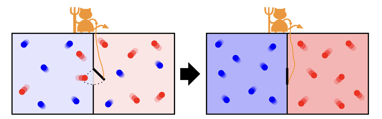
Maxwell’s demon controlling the door that allows the passage of single molecules from one side to the other. The initial hot gas gets hotter at the end of the process while the cold gas gets colder.
Maxwell’s Demon:
Maxwell’s Demon is a thought experiment that challenges the second law of thermodynamics by envisioning a tiny being capable of sorting molecules based on their speeds. By selectively allowing faster or slower molecules to pass through a gate, the demon appears to reduce entropy without expending energy. However, the act of gathering and processing information incurs a thermodynamic cost, ensuring that the overall entropy balance is maintained. This paradox underscores that information is a physical quantity with measurable effects on energy and entropy.
Maximum Entropy (MaxEnt) Principle
Probability represents our incomplete information. Given partial knowledge about some variables how should we construct a probability distribution that is unbiased beyond what we know?
The Maximum Entropy (MaxEnt) Principle provides the best approach: we choose probabilities to maximize Shannon entropy while satisfying given constraints.
This ensures the least biased probability distribution possible, consistent with the available information.
We seek to maximize subject to the constraints:
To enforce these constraints, we introduce Lagrange multipliers , leading to the Lagrangian (also called the objective function):
To maximize , we take its functional derivative with respect to :
Since is simply a constant normalization factor, we define and arrie at final expression for probability distribution:
Interperation of MaxEnt
The probability distribution takes an exponential form in the constrained variables .
The normalization constant (also called the partition function) ensures that the probabilities sum to 1.
The Lagrange multipliers encode the specific constraints imposed on the system.
This result is fundamental in statistical mechanics, where it leads to Boltzmann distributions, and in machine learning, where it underpins maximum entropy models.
Application MaxEnt: Biased Die Example
If we are given a fair die MaxENt would predict as there are no constraints.
But suppose we are given a biased die the average outcome of which is rolling on average a number . The entropy function to maximize becomes:
Solving the variational equation, we find that the optimal probability distribution follows an exponential form:
where is the partition function ensuring normalization:
To determine , we use the constraint :
This equation can be solved numerically for . In many cases, Newton’s method or other root-finding techniques can be employed to find the exact value of . This distribution resembles the Boltzmann factor in statistical mechanics, where higher outcomes are exponentially less probable.
Source
import numpy as np
from scipy.optimize import root
import matplotlib.pyplot as plt

x = np.arange(1, 7)
target_mean = 4.2

def maxent_prob(lambdas):
    lambda1 = lambdas[0]
    Z = np.sum(np.exp(-lambda1 * x))
    return np.exp(-lambda1 * x) / Z

def constraint(lambdas):
    p = maxent_prob(lambdas)
    mean = np.sum(x * p)
    return [mean - target_mean]

# Solve for lambda
sol = root(constraint, [0.0])
lambda_opt = sol.x[0]

# Optimal distribution
p_opt = maxent_prob([lambda_opt])

print(f"λ1 = {lambda_opt:.4f}")
for i, p in enumerate(p_opt, 1):
    print(f"P({i}) = {p:.4f}")

# Plot
plt.bar(x, p_opt, edgecolor='black')
plt.title("MaxEnt Distribution (Mean Constraint Only)")
plt.xlabel("Die Outcome")
plt.ylabel("Probability")
plt.xticks(x)
plt.grid(axis='y', linestyle='--', alpha=0.6)
plt.show()
λ1 = -0.2490
P(1) = 0.0818
P(2) = 0.1050
P(3) = 0.1347
P(4) = 0.1727
P(5) = 0.2216
P(6) = 0.2842

Relative Entropy
In the MaxEnt derivation, we implicitly maximized entropy relative to an underlying assumption of equal-probability microstates. We now make this idea precise.
Consider a 1D Brownian particle starting at and diffusing freely. Its probability distribution at time (t) is Gaussian:
The Shannon entropy of this distribution is
which evaluates to
suggesting that entropy grows as the particle spreads in space.
Problem: Grid Dependence of Shannon Entropy
For continuous variables, Shannon entropy is not absolute: it depends on the choice of spatial resolution (\Delta x). Refining the grid causes (S) to diverge, making it unsuitable for comparing entropy across different distributions or times.
To obtain a well-defined, resolution-independent measure, we instead use relative entropy.
Relative entropy quantifies the information cost of using when the system is actually distributed as . It is non-negative and vanishes if and only if .
Quantifying entropy of regions A and B
Let (X) be a random variable with distribution . Partition its domain into two disjoint regions (A) and (B).
Probabilities (weights)
Conditional (within-region) entropies would then be:
These quantify intrinsic spread / heterogeneity within each region, independent of how often the region is occupied.
Macro (between-region) entropy
Define a coarse-grained variable (M \in {A,B}).
This quantifies uncertainty about which region the system is in.
Exact entropy decomposition
$$ \boxed{ H(X) = H(M)
P_A H_A
P_B H_B } $$
Total entropy = between-region uncertainty + weighted within-region uncertainty.
: uncertainty between regions A and B
: uncertainty within regions (conditional entropies)
: weights that tell how much each region contributes
Asymmetry of KL Divergence and Irreversibility
Consider two normal distributions,
The KL divergence can be computed analytically:
$$ D_{\mathrm{KL}}(P|Q) = \ln\frac{\sigma_2}{\sigma_1}
\cdot \frac{\sigma_1^2+(\mu_1-\mu_2)^2}{2\sigma_2^2}
\frac{1}{2}. $$
This expression is not symmetric under , highlighting that KL divergence defines a directed notion of distance between distributions.
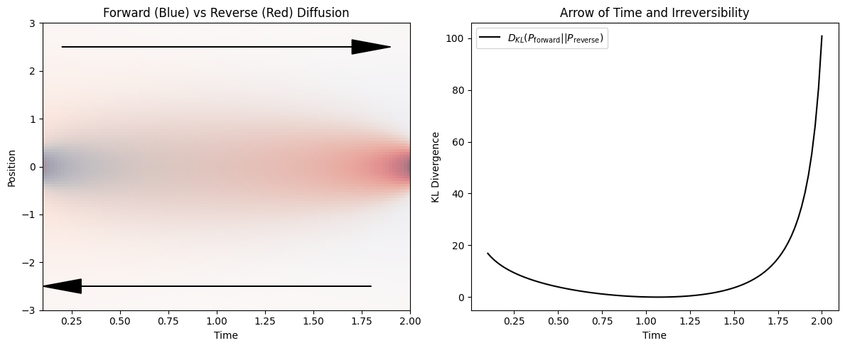
For diffusion, the probability distribution at time is Gaussian with variance . Comparing distributions at two times and yields:
This quantity is strictly positive unless (t_1=t_2).
Physical Interpretation of relative entropy
KL divergence measures the statistical distinguishability between probability distributions. For diffusion, the forward process (spreading in time) is statistically distinguishable from the hypothetical time-reversed process (spontaneous contraction).
This asymmetry reflects irreversibility: diffusion naturally increases entropy, while its time-reversed counterpart is overwhelmingly improbable.
This statistical asymmetry underlies the thermodynamic arrow of time.
Source
import numpy as np
import matplotlib.pyplot as plt

# Define time points
t_forward = np.linspace(0.1, 2, 100)
t_reverse = np.linspace(2, 0.1, 100)

# Define probability distributions for forward and reverse processes
x = np.linspace(-3, 3, 100)
sigma_forward = np.sqrt(t_forward[:, None])  # Diffusion spreads over time
sigma_reverse = np.sqrt(t_reverse[:, None])  # Reverse "contracts" over time

P_forward = np.exp(-x**2 / (2 * sigma_forward**2)) / (np.sqrt(2 * np.pi) * sigma_forward)
P_reverse = np.exp(-x**2 / (2 * sigma_reverse**2)) / (np.sqrt(2 * np.pi) * sigma_reverse)

# Compute Kullback-Leibler divergence D_KL(P_forward || P_reverse)
D_KL = np.sum(P_forward * np.log(P_forward / P_reverse), axis=1)

# Plot the distributions and KL divergence
fig, ax = plt.subplots(1, 2, figsize=(12, 5))

# Plot forward and reverse distributions
ax[0].imshow(P_forward.T, extent=[t_forward.min(), t_forward.max(), x.min(), x.max()], aspect='auto', origin='lower', cmap='Blues', alpha=0.7, label='P_forward')
ax[0].imshow(P_reverse.T, extent=[t_reverse.min(), t_reverse.max(), x.min(), x.max()], aspect='auto', origin='lower', cmap='Reds', alpha=0.5, label='P_reverse')

ax[0].set_xlabel("Time")
ax[0].set_ylabel("Position")
ax[0].set_title("Forward (Blue) vs Reverse (Red) Diffusion")
ax[0].arrow(0.2, 2.5, 1.5, 0, head_width=0.3, head_length=0.2, fc='black', ec='black')  # Forward arrow
ax[0].arrow(1.8, -2.5, -1.5, 0, head_width=0.3, head_length=0.2, fc='black', ec='black')  # Reverse arrow

# Plot KL divergence over time
ax[1].plot(t_forward, D_KL, label=r'$D_{KL}(P_{\mathrm{forward}} || P_{\mathrm{reverse}})$', color='black')
ax[1].set_xlabel("Time")
ax[1].set_ylabel("KL Divergence")
ax[1].set_title("Arrow of Time and Irreversibility")
ax[1].legend()

plt.tight_layout()
plt.show()
Relative Entropy in Machine Learning
If assigns very low probability where is large, the term becomes large, strongly penalizing underestimation of the data distribution.
If is broader than and assigns probability to unlikely regions, the penalty is mild because is small there.
As a result, KL divergence is asymmetric and not a true distance metric.
It penalizes missing probability mass far more than wasting probability mass, which is why it is widely used in machine learning and statistical inference.
Source
import numpy as np
import matplotlib.pyplot as plt
import ipywidgets as widgets
from ipywidgets import interact
from scipy.stats import norm

def plot_gaussians(mu1=0, sigma1=1, mu2=1, sigma2=2):
    x_values = np.linspace(-5, 5, 1000)  # Define spatial grid
    P = norm.pdf(x_values, loc=mu1, scale=sigma1)  # First Gaussian
    Q = norm.pdf(x_values, loc=mu2, scale=sigma2)  # Second Gaussian

    # Avoid division by zero in KL computation
    mask = (P > 0) & (Q > 0)
    D_KL_PQ = np.trapezoid(P[mask] * np.log(P[mask] / Q[mask]), x_values[mask])  # D_KL(P || Q)
    D_KL_QP = np.trapezoid(Q[mask] * np.log(Q[mask] / P[mask]), x_values[mask])  # D_KL(Q || P)

    # Plot the distributions
    plt.figure(figsize=(8, 6))
    plt.plot(x_values, P, label=fr'$P(x) \sim \mathcal{{N}}({mu1},{sigma1**2})$', linewidth=2)
    plt.plot(x_values, Q, label=fr'$Q(x) \sim \mathcal{{N}}({mu2},{sigma2**2})$', linewidth=2, linestyle='dashed')
    plt.fill_between(x_values, P, Q, color='gray', alpha=0.3, label=r'Difference between $P$ and $Q$')

    # Annotate KL divergences
    plt.text(-4, 0.15, rf'$D_{{KL}}(P || Q) = {D_KL_PQ:.3f}$', fontsize=12, color='blue')
    plt.text(-4, 0.12, rf'$D_{{KL}}(Q || P) = {D_KL_QP:.3f}$', fontsize=12, color='red')

    # Labels and legend
    plt.xlabel('$x$', fontsize=14)
    plt.ylabel('Probability Density', fontsize=14)
    plt.title('Interactive KL Divergence Between Two Gaussians', fontsize=14)
    plt.legend(fontsize=12)
    plt.grid(True)
    plt.show()

interact(plot_gaussians,
         mu1=widgets.FloatSlider(min=-3, max=3, step=0.1, value=0, description='μ1'),
         sigma1=widgets.FloatSlider(min=0.1, max=3, step=0.1, value=1, description='σ1'),
         mu2=widgets.FloatSlider(min=-3, max=3, step=0.1, value=1, description='μ2'),
         sigma2=widgets.FloatSlider(min=0.1, max=3, step=0.1, value=2, description='σ2'))

<function __main__.plot_gaussians(mu1=0, sigma1=1, mu2=1, sigma2=2)>Protein Sequences, Evolution, and Entropy
1. Sequence Conservation as Low Entropy
Protein sequences evolve under functional and structural constraints. At each sequence position (i), amino-acid usage is described by a probability distribution (p_i(a)).
The site entropy
measures variability at that position.
Low entropy → strong evolutionary conservation (few amino acids tolerated)
High entropy → weak constraint (many amino acids allowed)
Conserved sites often correspond to active sites, binding interfaces, or structural cores.
2. Coevolution as Shared Constraint
Some positions are not conserved individually but are correlated across evolution.
For two positions , define a joint distribution . Their mutual information
quantifies coevolution.
High : mutations at depend on mutations at
Indicates structural contacts, compensatory mutations, or allosteric coupling
Coevolution reflects constraints on combinations, not individual residues.
3. Entropy Reduction by Function
Evolution does not minimize entropy everywhere—it redistributes it.
Functional requirements reduce entropy at critical sites
Flexibility and robustness allow entropy elsewhere
Coevolution preserves function while permitting sequence diversity
Thus, proteins balance:
4. Big Picture
Entropy quantifies how many sequences are compatible with function
Conservation identifies where entropy is suppressed
Coevolution reveals how entropy is shared across positions
Evolution sculpts protein sequences by concentrating entropy away from functionally critical degrees of freedom.
Problems
Problem-1: Compute Entropy for gas partitioning
A container is divided into two equal halves. It contains 100 non-interacting gas particles that can freely move between the two sides. A macrostate is defined by the fraction of particles in the right half .
Write down an exprssion for entropy S(f)
Consult the section on Random Walk and Combinatorics formula
Evaluate for:
(10% left, 90% right)
(25% left, 75% right)
(50% left, 50% right)
Relate entropy to probability using Large Deviation Theory and answer the following questions:
Which macrostate is most probable?
How does entropy influence probability?
Why are extreme fluctuations (e.g., ) unlikely?
Problem-2: Guassians in 2D
Below we generate three 2D gaussians with varying degree of correltion betwene and . Run the code to visualize
import numpy as np
import matplotlib.pyplot as plt

# Define mean values
mu_x, mu_y = 0, 0  # Mean of x and y

# Define standard deviations
sigma_x, sigma_y = 1, 1  # Standard deviation of x and y

# Define different correlation coefficients
correlations = [0.0, 0.5, 0.9]  # Varying degrees of correlation

# Generate and plot 2D Gaussian samples for different correlations
fig, axes = plt.subplots(1, 3, figsize=(15, 5))

for i, rho in enumerate(correlations):
    # Construct covariance matrix
    covariance_matrix = np.array([[sigma_x**2, rho * sigma_x * sigma_y],
                                   [rho * sigma_x * sigma_y, sigma_y**2]])

    # Generate samples from the 2D Gaussian distribution
    samples = np.random.multivariate_normal([mu_x, mu_y], covariance_matrix, size=1000)

    # Plot scatter of samples
    axes[i].scatter(samples[:, 0], samples[:, 1], alpha=0.5)
    axes[i].set_title(f"2D Gaussian with Correlation ρ = {rho}")
    axes[i].set_xlabel("X")
    axes[i].set_ylabel("Y")

plt.tight_layout()
plt.show()
Compute entropy using probability distributions and
Compute relative entropy which is known as Mutual Information. How can you interpret this quantity
You will need these functions. Also check out
scipy.stats.entropy
| Task | numpy Function |
|---|---|
| Compute histogram for | numpy.histogram2d |
| Compute histogram for , | numpy.histogram |
| Normalize histograms to get probabilities | numpy.sum() |
| Compute entropy manually | numpy.log(), numpy.sum() |
Problem-3: Gambling with ten sided die
Take a ten sided die described by random variable
Experiment shows that after many throughs the average number die shows is with variance .
Determine probabilities of ten die sides . You can use the code for six sided die in this notebook. But remember there are now two constraints one on mean and one on variance!
Problem-3 Biased Random walker in 2D
A random walker moves on a 2D grid, taking steps in one of four possible directions:
Each step occurs with unknown probabilities:
which satisfy the normalization condition:
Experimental measurements indicate the expected displacement per step:
Using the Maximum Entropy (MaxEnt) principle, determine the probabilities by numerically solving an optimization problem.
You will need
scipy.minimize(entropy, initial_guess, bounds=bounds, constraints=constraints, method='SLSQP')to do the minimization. Check the documentation to see how it works
Problem-5: Arrow of time in 2D diffusion
Simulate 2D diffusion using a Gaussian distribution
Model diffusion in two dimensions with a probability distribution:
Generate samples at different time steps using
numpy.random.normalwith time-dependent variance.
Compute the relative entropy as a function of time
Use relative entropy (Kullback-Leibler divergence) to compare the probability distributions at time with a reference time :
Compare forward and reverse evolution of diffusion
Compute the relative entropy between forward () and reverse () diffusion distributions.
Quantify how diffusion leads to irreversible evolution by evaluating:
Interpret the results
How does relative entropy change with time?
Why is the forward process distinguishable from the reverse process?
What does this tell us about the arrow of time?