Probability theory#
What you need to know
Sample space \(\Omega\) is a set of elementary outcomes or events.
Events can contain more than one elementary event and can be constructed by forming subsets (\(A\), \(B\), \(C\) etc) of \(\Omega\)
Probability function P(A) assigns a numeric value to each event, A quantifying certainty of an event happening on a 0-1 scale.
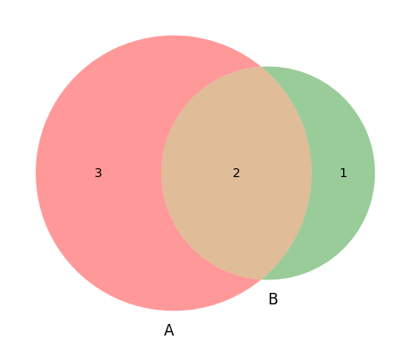
Venn diagrams visualize P(A) as a “volume fraction” of our confidence in the event expressed on 0-1 scale.
Probability axioms define a set of logical rules for creating composite events from trivial ones.
Bayesian approach: In physical sciences and modeling one often deals with situations where counting is impossible. Hence, probability is interpreted as a degree of belief.
Probabilistic world of complex many particle systems#
Fig. 1 Characterizing many particle complex systems is best done via probabilistic approach.#
What is the probability to find a gas in upper right corner cell?
What is the probability that all gas atoms will be in left side of the box?
What is the probability distribution of velocities of the gas?
Fig. 2 Simulations of a Random Walk in 1D#
What is the probability of finding molecule away from center by n steps out of N?
How do we obtain probability distribution after N steps given probability for 1 step?
Why is there tendency for probability distributions to evolve towards Gaussian?
Sample space#
The sample space, often signified by an \(\Omega\) is a set of all possible elementary events.
Elementary means the events can not be further broken down into simpler events. For instance, rolling a die can result in any one of six elementary events.
States of \(\Omega\) are sampled during a system trial, which could be done via an experiment or simulation.
If our trial is a single roll of a six-sided die, then the sample has size \(n(\Omega) = 6\)
A fair coin is tossed once has a sample size \(n(\Omega) = 2\)
If a fair coin is tossed three times in a row, we will have sample space of size \(n(\Omega) = 2^3\)
Position of an atom in a container of size \(L_x\) along x. \(n(\Omega)\) is a huge number. We will need some special tools to quantify.
Events, micro and macro states#
An event in probability theory refers to an outcome of an experiment. Event can contain one or more elementary events from \(\Omega\).
Event can be getting getting 5 on a die or getting any number less than 5.
In the context of statistical mechanics, we are going to call elementary events in \(\Omega\) microstates and events containing multiple microstates as macrostates
If we roll a single die there are six micostates. We can define a macrostate as an event \(A\) of getting any number less than 4
\[A= \{1, 2, 3 \}\]Or we can create a macrostate \(B\) containing only even numbers
\[B = \{2, 4, 6 \}\]IF we roll toss two coins microstates are HT, TH, HH, TT. We can define a macrostate \(D\) of having 50% H and 50% T
\[D = \{TH, HT\}\]A microstate of a gas atom in 1D container could be its position x. A macrostate could be finding atom anywehere in the second half of the container
\[C = \{L_x/2, ..., L_x \} \]
Compute probabilities through counting#
probabilities of events as fractions in the sample space
\(n(A)\) probability of event, e.g rolling an even number. The size of the event space is 3
\(n(\Omega)\) size of sample space. In the context of single die roll is equal 6
Visualizing events as Venn diagrams#
# COllab has this but in local notebook you may want to install it
#!pip install matplotlib-venn #install if running locally
import matplotlib_venn as venn
import matplotlib.pyplot as plt

Omega = {1,2,3,4,5,6}

A = {1, 2, 3, 4, 5}

B = {4, 5, 6}

venn.venn2([A, B], set_labels=('A','B'))

print(len(A)/len(Omega))
print(len(B)/len(Omega))
print(len(A & B)/len(Omega))
print(len(A | B)/len(Omega))
0.8333333333333334
0.5
0.3333333333333333
1.0
Probability Axioms#
Positivity and Normalization
Probability of rolling each number is 1/6 and rolling any number is 1.
Addition rule
For any sequence of mutually exclusive events, \(A_i \cap A_j = \emptyset \), the probability of their union is the sum of their probabilities,
Probability of die rolling even number is: \(1/6+1/6+1/6\)
Product rule
When independent events \(A_i \cap A_j = \emptyset\), the probability of their intersection is a product of their probabilities
Probability of rolling twice getting 3 and 5 is: \(\frac{1}{6}\cdot \frac{1}{6}\)
Complement
Given that \(A \cap \bar A=\emptyset\) and \(A \cup \bar A=\Omega\).
the probability of not rolling a number: \(1-\frac{1}{6}\)
Conditional probability and Bayes Theorem
Knowledge of past events may change the probability of future events
the probability of getting 4 given that we have rolled an even number: \(p(4|even) = \frac{p(even|4)p(4)}{p(even)}=\frac{1\cdot 1/6}{1/2}=1/3\)
Bayes Theorem#
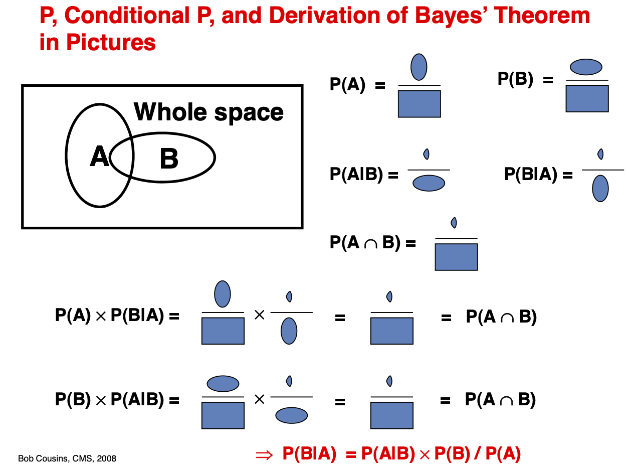
Fig. 3 Joint Probability \(P(A,B)\): Quantifies the probability of two or more events happening simultaneously. Marginal Probability \(P(A)\): Quantifies the probability of an event irrespective of the outcomes of other random variables. Is obtained by marginalization, summing over all possibilities of B. Conditional Probability \(P(A|B)\): Quantifies probability of event A given the information that event B happened.#
Example of Using Bayes Formula to Test Hypothesis
A test for cancer is known to be 90% accurate either in detecting cancer if present or in giving an all-clear if cancer is absent.
The prevalence of cancer in the population is 1%. How worried should you be if you test positive? Try answering this question using Bayes’ theorem.
Solution
Accuracy of a test (how often positives show up when cancer is certain)
Only 1% of the population has cancer; hence, we get the probability of an individual having (not having) cancer as:
Now we have all terms to compute \(p(X|+)\) probability of disease given the positive test.
Prior, Posterior, and Likelihood
Bayes’ theorem provides a powerful framework for testing hypotheses or learning model parameters from data. While the mathematical formulation remains the same, the terminology used in Bayesian inference differs from the standard probability notation:
where:
Prior: \(P(\theta)\) represents our initial belief about the hypothesis or parameter before observing the data. For example, if we are tossing a coin, a reasonable prior might be a gaussian centered at \(1/2\) or take unifrom distribution in absence of information.
Evidence: \(P(D)\) is the probability of the observed data, also known as the marginal likelihood. It accounts for all possible parameter values and normalizes the posterior. For example, it is the probability of obtaining a specific sequence, such as \(HTHH\), given all possible biases of the coin.
Likelihood: \(P(D | \theta)\) describes how probable the observed data is for a given parameter \(\theta\). E.g for sequence of \(HTHH\) it will be \(L(\theta)=\theta^3(1-\theta)\) giving probability of landing three H and 1 T.
Posterior: \(P(\theta | D)\) is the updated probability of the hypothesis after incorporating the observed data. This is the key quantity in Bayesian inference, as it represents our revised belief about \(\theta\) given the data. We can take value of \(\theta\) corresponding to maximum of posterior to be most likely value of our parameter. For our case of uniform prior and likelhood the maxima will be \(\theta = 3/4\) as we may expect.
Computing number of microstates via combinatorics#
Binomial Distribution (Two-State Systems)
When molecules can be in two states (e.g., adsorbed vs. free, spin-up vs. spin-down), the number of ways to arrange \(N\) molecules into state A \(k\) and state B \(N-k\) follows:
For example, if \(N\) gas molecules distribute between two parts of the box or spins occupying two energy levels, this formula gives the number of microstates for a given occupation \(k\).
Multinomial Distribution (Multiple States)
For systems with more than two states, such as molecules distributed among \(m\) energy levels, the number of ways to assign \(N\) molecules into states \(n_1, n_2, ..., n_m\) with \(\sum n_i = N\) is:
Example: partitioning gas particles
Consider a container filled with 1000 atoms of Ar.
What is the probability that the left half has 400 atoms?
What is the probability that the left half has 500 atoms?
: ::
What is a probability that 1/3 has 100 next 1/3 has 200 and next 1/3 has 700?
What is the total number of all possible partitionings or states of gas atoms in a container?
Each N lattice site in the container can be vacant or filled with \(2^N\) states.
Example: spins
Solid metal has 100 atoms. Magnetic measurements show that there are 10 atoms with spin down. If ten atoms are chosen at random, what is the probability that they all have spin up?
Solution
The total number of ways to choose any 10 atoms out of 100, regardless of spin is:
The number of ways to choose 10 atoms out of 90 with spin up is: $\(n(up) = \frac{90!}{10!(80)!}\)$
Probability of picking 10 up spins is:
def gas_partition(k1=30, k2=30, k3=30):
    '''partitioning N gas molecules into regions k1, k2 and k3'''

    from scipy.special import factorial

    N = k1+k2+k3

    return factorial(N) / (factorial(k1) * factorial(k2)* factorial(k3))

print( gas_partition(k1=50, k2=50, k3=0) )

print( gas_partition(k1=50, k2=49, k3=1) )

print( gas_partition(k1=50, k2=25, k3=25) )

print( gas_partition(k1=34, k2=33, k3=33) )
1.0089134454556417e+29
5.0445672272782094e+30
1.2753736048324953e+43
4.19244792425583e+45
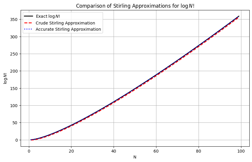
Strinling approximation of factorial and binomials#
Stitrling approximation of N!
This is the crude version of Stirling approximation that works out for \(N\gg 1\)
A more accurate version is:
Show code cell source
import numpy as np
import matplotlib.pyplot as plt
import scipy.special as sp

# Define range for N
N_values = np.arange(1, 100, 1)

# Exact factorial using log(N!)
log_fact_exact = np.log(sp.factorial(N_values))

# Crude Stirling approximation
log_fact_crude = N_values * np.log(N_values) - N_values

# More accurate Stirling approximation
log_fact_accurate = N_values * np.log(N_values) - N_values + 0.5 * np.log(2 * np.pi * N_values)

# Plot comparisons
plt.figure(figsize=(10, 6))
plt.plot(N_values, log_fact_exact, label="Exact $\log N!$", color="black", linewidth=2)
plt.plot(N_values, log_fact_crude, label="Crude Stirling Approximation", linestyle="--", color="red", linewidth=2)
plt.plot(N_values, log_fact_accurate, label="Accurate Stirling Approximation", linestyle=":", color="blue", linewidth=2)

plt.xlabel("N")
plt.ylabel("$\log N!$")
plt.title("Comparison of Stirling Approximations for $\log N!$")
plt.legend()
plt.grid(True)
plt.show()
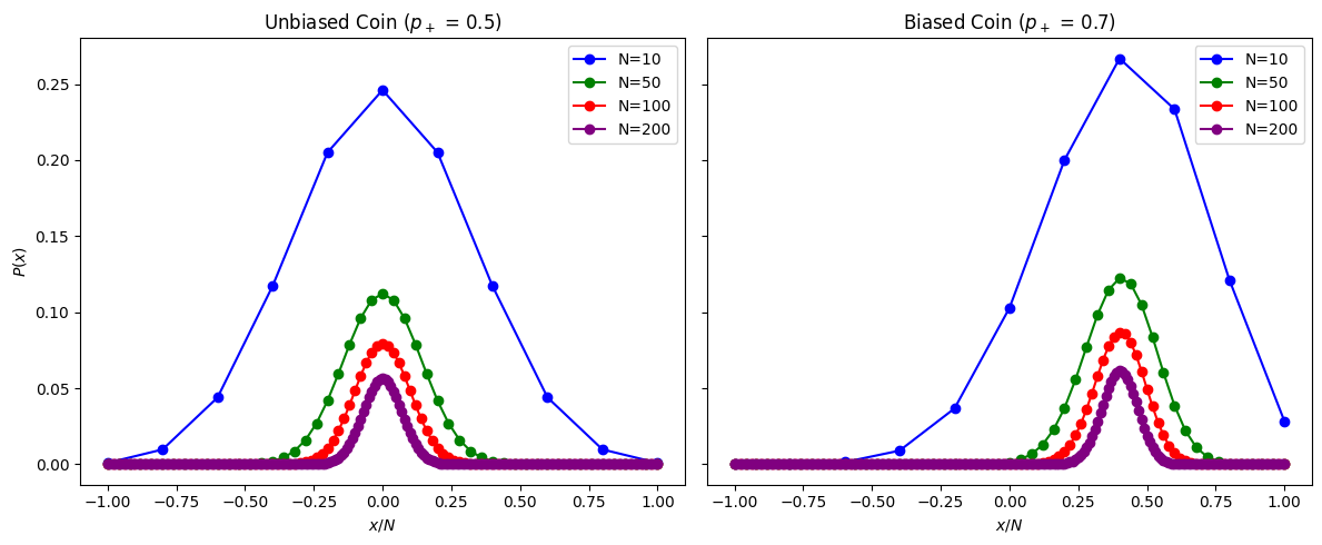
Random Walk#
Consider a problem with a binary outcome, with fixed probabilities \(p_{+} + p_{-} = 1\).
A clssic example is Random walk of N steps where molecules jumps right (\(+1\)) or left (\(-1\)) with fixed probabilities.
Other examples are tossing \(N\) coins or counting \(N\) non-interacting molecules in the left vs right hand side of a container.
Each experiment generates a sequence—e.g., \(+1, -1, -1, -1, +1\) for a random walk or \(HTHTTT\) for coin flips.
Such a sequence represents a single microstate in the sample space of all possible sequences which is \(\Omega=2^N\).
For unbiased random walk \(p_{+} = p_{-} = 1/2\), all microstates are equally probable and equal to \(\frac{1}{2^N}\).
For biased random walk \(p_{+} \neq p_{-}\) the probability of microstates (sequence) is determined by the product of step probabilities (becasue steps are independent)
Probability of a sequence (microstate)
A more interesting question is the probability of taking \(N_{+}\) steps to the right, or having a net displacement of \(\Delta N \), regardless of the sequence of events.
Probability of net number of steps or displacements (macrostate)
Probability of \(N_{+}\) Steps to the Right
Probability of \(\Delta N\) net displacement from the origin
Show code cell source
import numpy as np
import matplotlib.pyplot as plt
from scipy.special import comb

def P_x(N, x, p_plus):
    """Computes the binomial probability P(x|N, p_+)"""
    if (N + x) % 2 != 0:  # Ensure x is valid (must be even relative to N)
        return 0
    k = (N + x) // 2
    return comb(N, k) * (p_plus ** k) * ((1 - p_plus) ** (N - k))

# Define parameters
p_plus_unbiased = 0.5  # Unbiased case
p_plus_biased = 0.7  # Biased case
N_values = [10, 50, 100, 200]  # Different N values

# Create a figure with two subplots
fig, axes = plt.subplots(1, 2, figsize=(12, 5), sharey=True)

# Colors for different N values
colors = ["blue", "green", "red", "purple"]

# Loop through different N values
for i, N in enumerate(N_values):
    x_vals = np.arange(-N, N + 1, 2)  # x values must be -N to N, in steps of 2
    x_norm = x_vals / N  # Normalize x by N

    # Compute probabilities using vectorized function
    P_unbiased = np.array([P_x(N, x, p_plus_unbiased) for x in x_vals])
    P_biased = np.array([P_x(N, x, p_plus_biased) for x in x_vals])

    # Plot lines
    axes[0].plot(x_norm, P_unbiased, marker="o", linestyle="-", label=f"N={N}", color=colors[i])
    axes[1].plot(x_norm, P_biased, marker="o", linestyle="-", label=f"N={N}", color=colors[i])

# Titles and labels
axes[0].set_title(f"Unbiased Coin ($p_+$ = {p_plus_unbiased})")
axes[0].set_xlabel("$x/N$")
axes[0].set_ylabel("$P(x)$")
axes[0].legend()

axes[1].set_title(f"Biased Coin ($p_+$ = {p_plus_biased})")
axes[1].set_xlabel("$x/N$")
axes[1].legend()

plt.tight_layout()
plt.show()
Log of Macrostate Probability, Entropy, and fluctuations#
The logarithm of the probability of a given macrostate, \( P(N_{+} | N, p_{+}) \), can be written as:
In simulations, we measure the fraction of steps
Fractions will fluctuate but, in the limit of an infinitely long simulation, should converge to the true probabilities \(f_{\pm} \to p_{\pm}\)
Since \( f_{+} + f_{-} = 1 \) and \( p_{+} + p_{-} = 1 \), we introduce the \(f = f_{+}, \quad p = p_{+}\) notation to simplify subsequent expressions
where:
\( S \) represents the entropy term, related to the number of ways to distribute steps,
\( E \) is an energy-like function governing the bias in step distribution.
Energy as a Measure of Bias#
Taking the logarithm of the probability factor results in an energy-like function \( \epsilon \), which introduces a bias that shifts the distribution left or right depending on the probabilities of left/right steps, \( p_{\pm} \), determined by microscopic details of the random walk.
Where \(\epsilon=E/N\) is energy term per step of a random walk.
When \( p = \frac{1}{2} \), there is no bias, and the energy simplifies to \(E = N \log 2\)
Entropy as the Logarithm of number of Microstates in a Macrostate#
The entropy term, related to the number of ways to distribute steps. Using Stringling approximation for the log we obtain:
where \( s(f)=S/N \) is the entropy per step of a random walk.
Entropy of a macrostate in \(N\)-Step Random Walk
Entropy of a macrostate defined by a fraction of steps \(f\) is:
Alternatively, in terms of the net displacement fraction \(x = 2f - 1\):
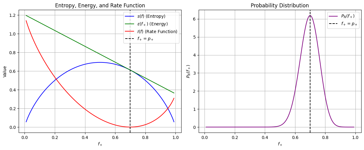
Large Deviation Theory#
By taking a log of macrostate probability \(P(f)\) we find that it scales linearly with \(N\) and is proportional to a \(I(f)\) which is independent of N
\[ \log P_{N}(f) \approx -N \Big[\epsilon(f) - s(f) \Big] = -N I(f). \]When there are \(N\) steps, molecules, or components, the probability distribution over the fraction of steps \(f\) tends to concentrate near the minima of \(I(f)\) caled Large deviation function
Large deviation function \(I\) dictates both the shape and decay of probability distributions in the large-\(N\) limit.
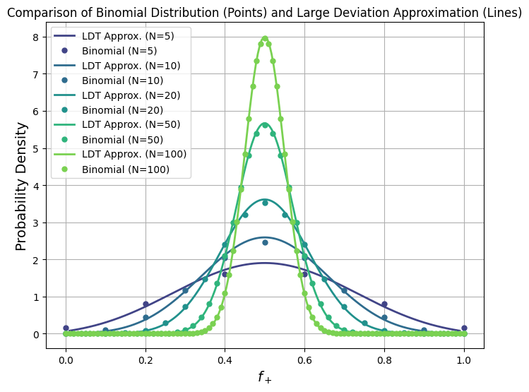
This general result applicable is known under the name of Large Deviation Theorem (LDT).
Large Deviation Theorem (LDT)
For a macrostate probability \(P(f)\) where \(f=n/N\) is some empirical fraction or mean quantity over \(N\) components:
\(I(f)\) is the rate function, which quantifies the likelihood of fluctuations away from the most probable value.
Example of \(I(f)\) for Random Walk: Determines how deviations of \(f_+\) (empirical fractions) from \( p_+\) (true or exact probabilities) are exponentially suppressed as \(N\) increases.
Show code cell source
# Re-import required libraries since execution state was reset
import numpy as np
import matplotlib.pyplot as plt

# Define parameters
p_plus = 0.7  # Biased probability
p_minus = 1 - p_plus  # Complementary probability

# Define range for f_+
f_plus_values = np.linspace(0.01, 0.99, 200)  # Avoid log(0) issues
f_minus_values = 1 - f_plus_values  # f_- = 1 - f_+

# Compute entropy component s(f_+)
s_values = -(f_plus_values * np.log(f_plus_values) + f_minus_values * np.log(f_minus_values))

# Compute energy component ε(f_+)
epsilon_values = - (f_plus_values * np.log(p_plus) + f_minus_values * np.log(p_minus))

# Compute large deviation rate function I(f_+)
I_values = f_plus_values * np.log(f_plus_values / p_plus) + f_minus_values * np.log(f_minus_values / p_minus)

# Compute probability P_N(f_+) using large deviation approximation
N = 50  # Arbitrary large N
P_x_values = np.exp(-N * I_values)  # Exponential suppression
P_x_values /= np.trapz(P_x_values, f_plus_values)  # Normalize for probability density

# Create subplots
fig, axes = plt.subplots(1, 2, figsize=(12, 5))

# First subplot: Entropy and Energy Components
axes[0].plot(f_plus_values, s_values, label=r"$s(f)$ (Entropy)", color="blue")
axes[0].plot(f_plus_values, epsilon_values, label=r"$\epsilon(f_+)$ (Energy)", color="green")
axes[0].plot(f_plus_values, I_values, label=r"$I(f)$ (Rate Function)", color="red")
axes[0].axvline(p_plus, linestyle="--", color="black", label=r"$f_+ = p_+$")
axes[0].set_xlabel(r"$f_+$")
axes[0].set_ylabel("Value")
axes[0].set_title("Entropy, Energy, and Rate Function")
axes[0].legend()
axes[0].grid()

# Second subplot: Probability Distribution P_N(f_+)
axes[1].plot(f_plus_values, P_x_values, label=r"$P_N(f_+)$", color="purple")
axes[1].axvline(p_plus, linestyle="--", color="black", label=r"$f_+ = p_+$")
axes[1].set_xlabel(r"$f_+$")
axes[1].set_ylabel(r"$P_N(f_+)$")
axes[1].set_title("Probability Distribution")
axes[1].legend()
axes[1].grid()

plt.tight_layout()
plt.show()
Show code cell source
import numpy as np
import matplotlib.pyplot as plt
from scipy.special import comb

def plot_large_deviation(N, theta, color):
    """Plots the large deviation approximation for given N and bias theta."""
    f = np.linspace(0.01, 0.99, 200)  # Avoid log(0) issues

    # Compute the rate function I(f)
    I = f * np.log(f / theta) + (1 - f) * np.log((1 - f) / (1 - theta))

    # Compute normalized probability P_LDT(f) ∼ exp(-N I(f))
    p_ldt = np.exp(-N * I)
    p_ldt /= np.trapz(p_ldt, f)  # Normalize using trapezoidal rule for integration

    plt.plot(f, p_ldt, color=color, linestyle="-", linewidth=2, label=f"LDT Approx. (N={N})")

def plot_binomial(N, theta, color):
    """Plots the exact binomial distribution for given N and bias theta."""
    n = np.arange(N + 1)
    f = n / N  # Convert discrete counts to fractions

    # Compute binomial probability mass function
    prob = comb(N, n) * theta**n * (1 - theta)**(N - n)

    # Normalize probability for direct comparison with LDT curve
    prob /= np.trapz(prob, f)

    plt.plot(f, prob, 'o', color=color, markersize=5, label=f"Binomial (N={N})")

# Parameters
theta = 0.5  # Fair coin
Ns = [5, 10, 20, 50, 100]  # Different values of N
colors = plt.cm.viridis(np.linspace(0.2, 0.8, len(Ns)))  # Use colormap for better distinction

# Create the plot
plt.figure(figsize=(8, 6))
for i, N in enumerate(Ns):
    plot_large_deviation(N, theta, colors[i])
    plot_binomial(N, theta, colors[i])

# Labels and formatting
plt.xlabel(r"$f_+$", fontsize=14)
plt.ylabel(r"Probability Density", fontsize=14)
plt.title("Comparison of Binomial Distribution (Points) and Large Deviation Approximation (Lines)", fontsize=12)
plt.legend(loc="upper left", fontsize=10)
plt.grid()
plt.show()
Gaussian Nature of Fluctuations#
The Taylor expansion of the large deviation function around its minimum leads to a Gaussian distribution in the limit of small fluctuations. This fundamental result in large deviation theory explains why fluctuations in equilibrium statistical mechanics are often Gaussian.
Let \( I(f) \) be the large deviation function, which attains a minimum at \( f_{\text{min}} \). Expanding around \( f_{\text{min}} \):
\[ I(f) = I(f_{\text{min}}) + \frac{1}{2} I''(f_{\text{min}}) (f - f_{\text{min}})^2 + \mathcal{O}((f - f_{\text{min}})^3). \]Since \( I(f_{\text{min}}) = 0 \) (by definition, probability is maximal at \( f_{\text{min}} \)), we obtain:
\[ I(f) \approx \frac{1}{2} I''(f_{\text{min}}) (f - f_{\text{min}})^2. \]Substituting this into the large deviation form:
\[ P(f) \approx e^{-N I(f)} \approx e^{-N \frac{1}{2} I''(f_{\text{min}}) (f - f_{\text{min}})^2} = e^{-\frac{(f - f_{\text{min}})^2}{2 \sigma^2}} \]where the variance is:
\[ \sigma^2 = \frac{1}{N I''(f_{\text{min}})}. \]This is a Gaussian distribution centered at \( f_{\text{min}} \), with variance \( \sigma^2 \). Here, \( f \) represents the fractional quantity \( f = n/N \), though one may also express the distribution in terms of absolute particle numbers, \( P(n) \).
Thus, the Taylor expansion of \( I(f) \) near its minimum shows that, for large \( N \), fluctuations become Gaussian, explaining why equilibrium statistical physics often exhibits Gaussian distributions.
Appendix: Explicit derivations#
Appendix A. Gaussian or large \(N\) limit of Binomial Distribution
The binomial distribution for large values of \(N\) has a sharply peaked distribution around its maximum (most likely) value \(\tilde{n}\). This motivates us to seek a continuous approximation by Taylor expanding the probability distribution around its maximum value \(\Delta n = n - \tilde{n}\) and keeping terms up to quadratic order.
Thus, from the onset, we aim for a Gaussian distribution. The task is to find the coefficients and justify that the third term in the Taylor expansion is negligible compared to the second.
We evaluate the derivative of \(\log n!\) in the limit of \(n \gg 1\) as:
We could also arrive at the same result by using Stirling’s approximation \(\log N! \approx N \log N - N\).
Taking the first derivative of the Taylor expansion for the binomial distribution, we find the peak of the distribution around which we expand:
We recall that \(\tilde{n} = N p\) is also the mean of the binomial distribution!
Having found the peak of the distribution and knowing the first derivative, we now proceed to compute the second derivative:
While the first derivative gave us the mean of the binomial distribution, we notice that the second derivative produces the variance \(\sigma^2 = N p (1 - p)\).
Now, all that remains is to plug the coefficients into our approximated probability distribution and normalize it. Why normalize? The binomial was already properly normalized, but since we made an approximation by neglecting higher-order terms, we must re-normalize.
Normalizing the Gaussian distribution is done via the following integral:
Finally, we obtain the normalized Gaussian approximation to the binomial distribution:
Appendix B. Poisson limit or the limit of large \(N\) and small \(p\) such that \(Np=const\)
This is a situation of rare events like rains in forest or radioactive decay of uranium where each individual event has small chance of happening \(p \rightarrow 0\) yet there are large number of samples \(N\rightarrow \infty\) such that one has a constant average rate of events \(\lambda = pN = const\)
In this limit distirbution is no longer well described by the gaussian as the shape of distribution is heavily skewed due to tiny values of p.
Writing factorial \(N!/(N-n)!\) explicitely we realize that it is dominated \(N^n\) and also \(N-n \approx N\)
Next let us plug in \(\lambda = pN = const\) and recall the definition of exponential \(lim_{x\rightarrow \infty }(1-1/x)^x = e^{-x}\)
Example of Gaussian limit of Large Deviation function for random walk
The large deviation rate function for a simple random walk is given by:
where \(f_+\) and \(f_-\) are empirical step probabilities, and \(p_+\), \(p_-\) are their expected values with \(p_+ + p_- = 1\).
Expansion Around the Minimum
The function \(I(f)\) is minimized at \(f_+ = p_+\), \(f_- = p_-\). Introducing small deviations \(\delta f\):
Expanding the logarithms:
Substituting into \(I(f)\), the linear terms cancel, and we obtain:
Gaussian Limit
By the large deviation principle:
This is a Gaussian with variance:
Thus, the empirical frequency \(f_+\) follows a Gaussian distribution in the large \(N\) limit.
Problems#
Problem 1: Counting Dies and coins#
You flip a coin 10 times and record the data in the form of head/tails or 1s and 0s
What would be the probability of ladning 4 H’s?
What would be the probability of landing HHHTTTHHHT sequence?
In how many ways can we have 2 head and 8 tails in this experiments?
Okay, now you got tired of flipping coins and decide to play some dice. You throw die 10 times what is the probability of never landing number 6?
You throw a die 3 times what is the probability of obtaining a combined sum of 7?
Problem 2: Counting gas molecules#
A container of volume \(V\) contains \(N\) molecules of a gas. We assume that the gas is dilute so that the position of any one molecule is independent of all other molecules. Although the density will be uniform on the average, there are fluctuations in the density. Divide the volume \(V\) into two parts \(V_1\) and \(V_2\), where \(V = V_1 + V_2\).
What is the probability p that a particular molecule is in each part?
What is the probability that \(N_1\) molecules are in \(V_1\) and \(N_2\) molecules are in \(V_2\)?
What is the average number of molecules in each part?
What are the relative fluctuations of the number of particles in each part?
Project Porosity of materials#
A simple model of a porous rock can be imagined by placing a series of overlap- ping spheres at random into a container of fixed volume \(V\) . The spheres represent the rock and the space between the spheres represents the pores. If we write the volume of the sphere as v, it can be shown the fraction of the space between the spheres or the porosity \(\phi\) is \(\phi =e^{-Nv/V}\), where \(N\) is the number of spheres.
For simplicity, consider a 2D system, (e.g \(v=\frac{1}{4}\pi d^2\), see wiki if you forgot the formula). Write a python function which place disks of \(d=1\) into a square box. The disks can overlap. Divide the box into square cells each of which has an edge length equal to the diameter of the disks. Find the probability of having 0, 1, 2, or 3 disks in a cell for \(\phi\) = 0.03, 0.1, and 0.5.
You will need np.random.uniform() to randomly place N disks of volume v into volume V. Check out this cool python lib for porosity evaluation of materials R Shkarin, et al Plos Comp Bio 2019