Thermodynamic Potentials - Statmech4ChemBio

Reversible Work Theorem¶

Consider two processes between the same initial and final states with a heat bath at temperature $T$ .
One process is irreversible The other is reversible. But Since both processes have the same energy change,

\Delta E = \delta W+ \delta Q = dW_{rev} + dQ_{rev}

(1)

Since $\delta Q_{rev} = TdS$ we can rewrite work in terms ofreversible work:

\delta W = dW_{rev} + TdS - dQ

(2)

Using Clausius inequality $TdS-\delta Q\geq 0$ we arrive at the relationship between irreversible and reversible work

\delta W \geq dW_{\text{rev}}

(3)

figure-md - Unknown Directive

<img src="./figs/polymer.png" class="bg-primary" width="500px">  

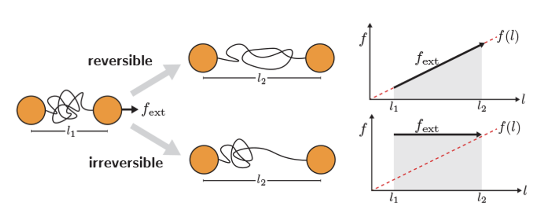
Comparison of a reversible and an irreversible pulling process of a chain molecule with a linear force-extension equation of state. the minimum work is achieved by reversible pulling and is equal to free energy difference.

Thus, the minimum work required for a transformation at constant $T$ is given by the reversible work.
For example, in a chain molecule with a linear force-extension equation of state, the work equal to the area under the force-extension curve is minimized when the force just suffices to induce the transition.
Writing reversible work in terms of a change of Energy and heat: $\delta W_{rev} = dE-TdS$ we see that under $T=const$ work is equal to a full differential

\delta W \geq dE - TdS = d(E-TS)

(4)

We call the quantity of $F=E-TS$ as Helmholtz free energy. Free energy differnece is the minimum amount of work that needs to be done on the syste to go from equilibrium state A to B.

W \geq \Delta F

(5)

If instead it is the system that is doing the work on the environment $W<0$ then the the Helmholtz free energy can bee seen as the maximum amount of energy available to do work to go from equilibrium state A to B.

|\Delta F| \geq |W|

(6)

Free Energy Minimization principle¶

When there is no work done $W=0$ which happens when fixing volume and temperature:

dF_{V,T} \leq 0

(8)

Thus, at fixed $T$ and $V$ , equilibrium is achieved when the Free Energy is at its minimum

Free Energy and the System-Centric Perspective

In thermodynamics, a system in contact with a thermal reservoir undergoes energy exchange, affecting both the system’s entropy $S$ and the reservoir’s entropy $S_{\text{res}}$ . Directly tracking these changes can be cumbersome. The adoption of free energy circumvents this issue by encapsulating the reservoir’s effects into a single function.
Consider the total entropy change in an isothermal process at temperature $T$ :

\Delta S_{\text{total}} = \Delta S + \Delta S_{\text{res}} \geq 0

(10)

Since the heat exchanged with the reservoir is $Q = \Delta U - W$ , where $U$ is internal energy and $W$ is work done on the system, the reservoir’s entropy change is:

\Delta S_{\text{res}} = -\frac{Q}{T} = -\frac{\Delta U - W}{T}

(11)

Thus, the total entropy change can be rewritten as:

\Delta S_{\text{total}} = \Delta S - \frac{\Delta U - W}{T}

(12)

Rearranging, we obtain:

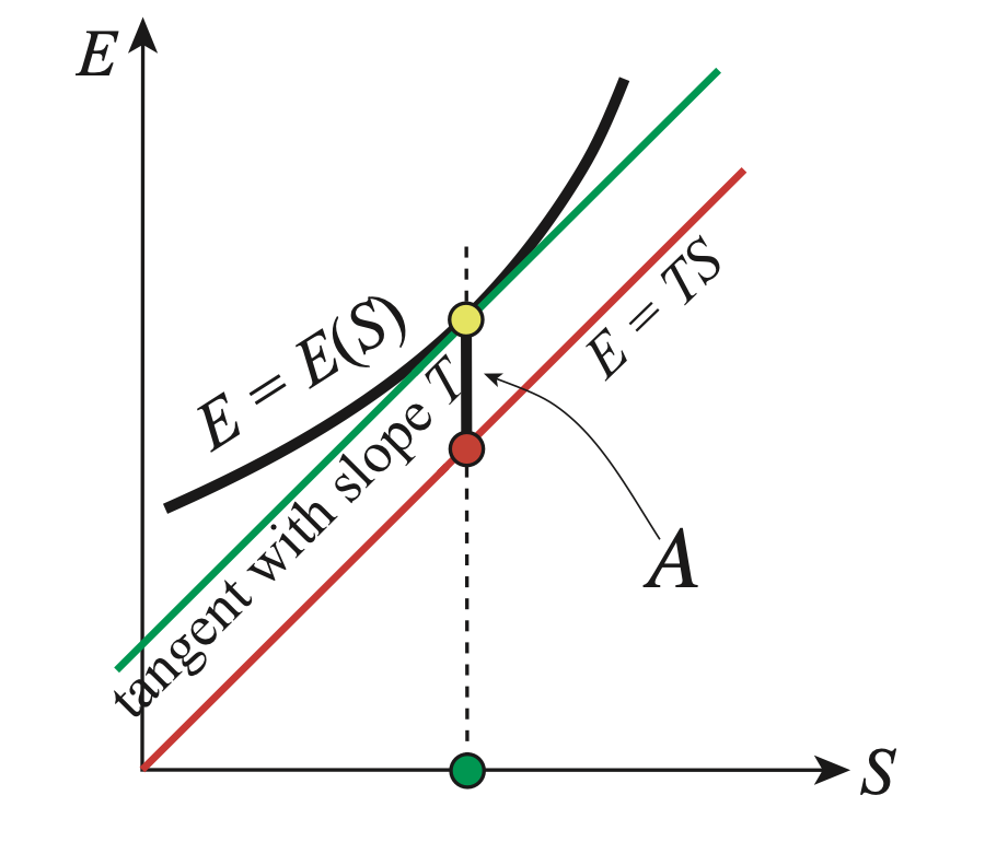
T \Delta S_{\text{total}} = T\Delta S - \Delta U + W

(13)

Defining the Helmholtz free energy $F = U - TS$ , we arrive at:

T \Delta S_{\text{total}} = W - \Delta F \geq 0

(14)

We arrive at reversible work theorem stating that work we do on the system goes into free energy change and the rest dissipated

\Delta F \leq W

(15)

For spontaneous processes at constant $T$ and volume ( $W = 0$ ), this simplifies to:

\Delta F \leq 0

(16)

This result shows that minimizing $F$ governs equilibrium and spontaneous evolution. The key advantage is that we focus only on the system’s free energy $F$ , avoiding explicit tracking of the entropy changes in the reservoir. This simplification makes free energy a powerful tool in equilibrium thermodynamics and statistical mechanics.

Free Energies and Legendre Transforms¶

Energy $E(S, V, N)$ is a natural function of extensive variables.
Equilibrium is found by minimizing $E$ with respect to its independent variables.
In experiments, it’s often more convenient to control intensive variables (e.g., $T$ , $P$ ) instead of extensive ones.
Legendre transforms allow us to switch from energy to free energies, which have more practical independent variables.
The transformation replaces extensive variables with their conjugate intensive variables, giving new thermodynamic potentials:

E(S, V, N) \rightarrow A(T, V, N) \quad \text{(Helmholtz Free Energy)}

(17)

E(S, V, N) \rightarrow G(T, P, N) \quad \text{(Gibbs Free Energy)}

(18)

E(S, V, N) \rightarrow \Omega(T, P, \mu) \quad \text{(Grand Potential)}

(19)

Legendre transform preserves convexity: equilibrium is still found by minimization.
Free energies contain the same information as $E$ since the transform is invertible.
Free energies use experimentally controllable variables (e.g., $T$ , $P$ ).

Helmholtz Free energy

E(N, V, S) \rightarrow E - T\cdot S = F(N, V, T)

(23)

Where energy and entropy are now expressed in terms of temperature $T=\frac{\partial E}{\partial S}$

dF = dE -d(TS) = dE - TdS - SdT

(24)

dF = -SdT - pdV + \mu dN

(25)

Gibbs Free energy

E(N, V, S) \rightarrow E - T\cdot S + p\cdot V = G(N, p, T)

(26)

Where energy, entropy volume are now expressed in terms of temperature $T=\frac{\partial E}{\partial S}$ and pressure $p=-\frac{\partial E}{\partial V}$

dG = dE -d(TS) + d(pV) = dE - TdS - SdT + pdV + Vdp

(27)

dG = -SdT + Vdp + \mu dN

(28)

Visualizing the Legendre Transform¶

Simply put, the Legendre transform replaces the variable $x$ in a function $f(x)$ with its derivative:
$y = \frac{df}{dx}.$
(29)
This results in a new function $g(y)$ , expressed in terms of the slope.

figure-md - Unknown Directive

<img src="./figs/Legendre.png" class="bg-primary" width="300px">  

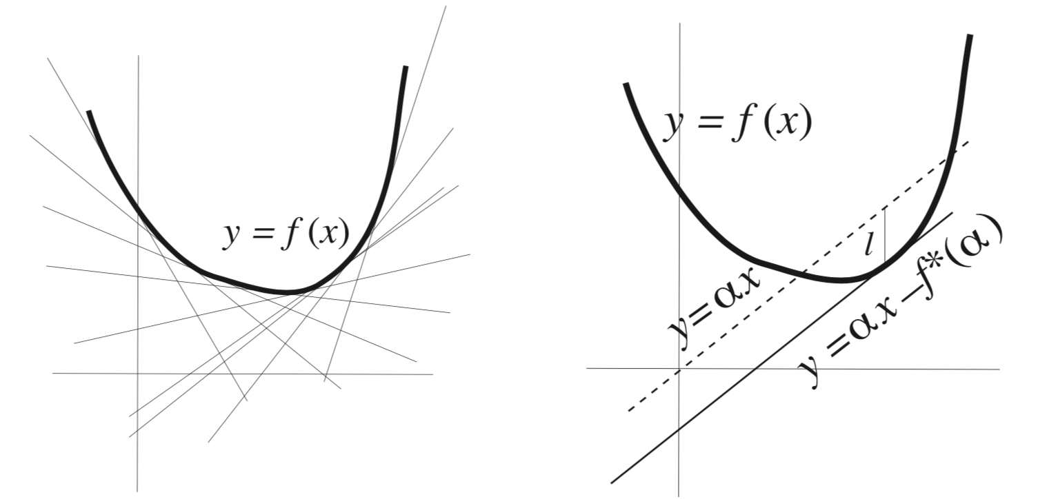
Visualizing a convex function and its legendre transform.

Geometric Intuition: A curve can be described either as a collection of points $(x, f(x))$ or as a collection of tangent slopes $y = df/dx$ .
- For this correspondence to be one-to-one, the function must be convex and have a well-defined minimum.
Legendre transform in general:
- It maps one convex function $f(x)$ to another convex function $f^*(\alpha)$ .
- Moreover, the transformation is involutive, meaning that applying it twice returns the original function.

Example of Legendre transform of 1D function

f(x) = x^2

(30)

a = f'(x) =2x \rightarrow x = a/2

(31)

g(\alpha) = f^*(\alpha) = max_x \Big[ \alpha x - f(x) \Big ] = \alpha^2/2 - \alpha^2/4 = \alpha^2/4

(32)

import numpy as np
import matplotlib.pyplot as plt
import matplotlib.animation as animation
from IPython.display import HTML
# Define the convex function (example: quadratic function f(x) = x^2)
def f(x):
    return x**2

def df_dx(x):
    return 2*x  # Derivative of f(x)

def legendre_transform(x):
    p = df_dx(x)
    g_p = p*x - f(x)
    return p, g_p

# Generate x values
x_vals = np.linspace(-2, 2, 100)
f_vals = f(x_vals)

# Create the figure
fig, ax = plt.subplots(1, 2, figsize=(10, 5))
ax[0].set_xlim(-2, 2)
ax[0].set_ylim(-1, 5)
ax[0].set_title("Function and Tangents")
ax[0].set_xlabel("x")
ax[0].set_ylabel("f(x)")
ax[0].plot(x_vals, f_vals, label="$f(x)$", color="blue")

ax[1].set_xlim(-4, 4)
ax[1].set_ylim(-2, 4)
ax[1].set_title("Legendre Transform")
ax[1].set_xlabel("p")
ax[1].set_ylabel("g(p)")

# Initialize elements for animation
point, = ax[0].plot([], [], 'ro', markersize=6)  # Moving point on f(x)
tangent_line, = ax[0].plot([], [], 'r-', lw=1)  # Tangent line
legendre_point, = ax[1].plot([], [], 'go', markersize=6)  # Points on g(p)
g_p_vals, p_vals = [], []  # Store computed values for g(p)

# Animation update function
def update(frame):
    x = -2 + frame * 0.05  # Move x from -2 to 2
    p, g_p = legendre_transform(x)
    tangent_x = np.linspace(x-1, x+1, 10)
    tangent_y = f(x) + df_dx(x) * (tangent_x - x)
    
    # Update primary function plot
    point.set_data([x], [f(x)])
    tangent_line.set_data(tangent_x, tangent_y)
    
    # Update Legendre transform plot
    p_vals.append(p)
    g_p_vals.append(g_p)
    legendre_point.set_data(p_vals, g_p_vals)
    
    return point, tangent_line, legendre_point

# Create animation
plt.legend()
ani = animation.FuncAnimation(fig, update, frames=80, interval=100, blit=True)
plt.close()
HTML(ani.to_jshtml())

Mathematical Formulation of Legendre Transform¶

The Legendre transform of $f(x)$ is given by:

f^*(\alpha) = \max_x \big[ \alpha x - f(x) \big].

(33)

Applying the transform again recovers the original function:

f(x) = \max_{\alpha} \big[ \alpha x - f^*(\alpha) \big].

(34)

In thermodynamis we are looking at minimum of energies and free energies. Hence we write Helmholtz Free energy as:

A = min_S[ E(S) - T S]

(35)

figure-md - Unknown Directive

<img src="./figs/Leg1.png" class="bg-primary" width="300px">  

Draw a line (red line) with the same slope passing through the origin, $E=TS$. Then, $A=E-TS$ is the $E$-coordinate value of the yellow dot subtracted that of the red dot. This implies that the minimum of the (signed) distance measured along the $E$-axis between the curve $E(S)$ and the line $E=TS$ is $A$

Problems¶

Problem 1: Legendre transforms and free energy calculations¶

Use Legendre transform to go from $E(N, V, T)$ to $F(S,p,N)$ and to $G(T,p,N)$ .
1 mole of an ideal gas at 300 K is quasistatically and isothermally compressed from 5 to 25atm. Find $\Delta F$ and $\Delta G$