The Inverse Transform of RVs - Statmech4ChemBio

%matplotlib inline

import numpy as np
import matplotlib.pyplot as plt
import seaborn as sns

The idea¶

Inverse transform sampling is a basic method for pseudo-random number sampling, i.e. for generating sample numbers at random from any probability distribution given its cumulative distribution function. That is, by drawing from a uniform distribution, we make it possible to draw from the other distribution in question.
Let’s start by defining uniform distribution $U(0,1)$ which generates random numbers $Z\sim U(0,1)$ falling on $[0,1]$ range. Now let’s look for a way of transforming random number $Z$ with $p(z)=\frac{1}{1-0}$ uniform pdf into a function $X(Z)$ where x is distributed according to some pdf $p(x)$ . The probability to find $x$ between $x$ and $x+dx$ is equal to:

p(x)dx = p(z)dz = dz

(1)

This relation is simply transform of variables. Now the key point to realize is that integrals from over $[-\infty, x(z)]$ for X and $[0, z]$ for Z are equal (these are cumulative distribution functions (CDF).

\int_{-\infty}^{x(z)} p(x') dx' = \int_0^z dz'= z

(2)

Thus, if we can (i) integrate expression on the left analytically and (ii) solve for $x$ then we are done! For most of the pdf at least one of the two is not possible. Below is a typical example where both (i) and (ii) states are easily done.

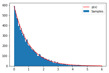
Example: Drawing from the exponential distribution.¶

For example, lets assume we would like to generate random numbers that follow the exponential distribution
$p(x) = \frac{1}{\lambda} e^{-x/\lambda}$
(3)
for $x\ge0$ and $f(x)=0$ otherwise. Following the recipe from the above we have

u = \int_{0}^{x} \frac{1}{\lambda} e^{-x'/\lambda} dx' = 1- e^{-x/\lambda}

(4)

Solving for $x$ we get

x = - \lambda \ln (1-u)

(5)

Formalized procedure:¶

Get a uniform sample $u$ from $U(0,1)$
Solve for $x$ yielding a new equation $x=F^{-1}(u)$ where $F$ is the CDF of the distribution we desire.
Repeat.

# Define the probability distribution function
p = lambda x: np.exp(-x)

# Compute its cumulative distribution function (CDF)
CDF = lambda x: 1 - np.exp(-x)

# Compute the inverse of the CDF
invCDF = lambda r: -np.log(1 - r)

# Define sampling limits
xmin, xmax = 0, 6  # Domain range
rmin, rmax = CDF(xmin), CDF(xmax)  # Range of CDF values

# Generate random samples
N = 10000
R = np.random.uniform(rmin, rmax, N)
X = invCDF(R)

# Compute histogram data
hist_vals, bin_edges = np.histogram(X, bins=100)

# Plot histogram of samples
plt.hist(X, bins=100, label='Samples', alpha=0.7, edgecolor='black')

# Overlay the theoretical probability density function (PDF)
x_vals = np.linspace(xmin, xmax, 1000)
plt.plot(x_vals, hist_vals[0] * p(x_vals), 'r', linewidth=2, label='p(x)')

# Display legend and formatting
plt.legend()
plt.xlabel('x')
plt.ylabel('Frequency')
plt.title('Inverse Transform Sampling of an Exponential Distribution')
plt.grid(alpha=0.3)
plt.show()