Estimating the pi by throwing pebbles on the sand
The key idea of this technique is that the ratio of the area of the circle to the square area that inscribes it is , so by counting the fraction of the random points in the square that are inside the circle, we get increasingly good estimates to .
Source
import numpy as np
import matplotlib.pyplot as plt

def circle_pi_estimate(N=10000, r0=1):
    """
    Estimate the value of pi using the Monte Carlo method.

    Generate N random points in a square with sides ranging from -r0 to r0.
    Count the fraction of points that fall inside the inscribed circle to estimate pi.

    Parameters:
    N (int): Number of points to generate (default: 10000)
    r0 (int): Radius of the circle (default: 1)

    Returns:
    float: Estimated value of pi
    """

    # Generate random points
    xs = np.random.uniform(-r0, r0, size=N)
    ys = np.random.uniform(-r0, r0, size=N)

    # Calculate distances from the origin and determine points inside the circle
    inside = np.sqrt(xs**2 + ys**2) < r0

    # Compute volume ratio as the ratio of points
    v_ratio = inside.sum() / N

    pi_estimate = 4 * v_ratio

    # Plotting
    fig, ax = plt.subplots(figsize=(6, 6))
    ax.plot(xs[inside], ys[inside], 'b.', label='Inside')
    ax.plot(xs[~inside], ys[~inside], 'r.', label='Outside')
    ax.set_title(f"Estimation of $\\pi$ = {pi_estimate}", fontsize=20)
    ax.set_xlabel("x")
    ax.set_ylabel("y")
    ax.legend()

    return pi_estimate
circle_pi_estimate(N=100000, r0=100)np.float64(3.13272)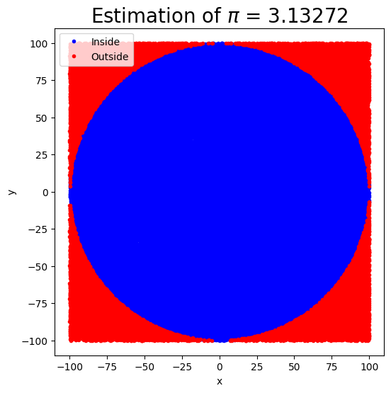
We will now use the same technique but compute a 1D definite integral from to by drawing a rectangle to cover the curve with dimensions and .
The area of the rectangle is . The area under the curve is .
If we choose a point uniformly at random in the rectangle, what is the probability that the point falls into the region under the curve? It is simply
Thus we can estimate the definite integral by drawing uniform points covering the rectangle and computing the integral as
Source
def myfunc1(x):
    return np.exp(-x)+ np.exp(-x)* x**2 * np.cos(x)**2 + np.exp(-2*x)*x**4* np.cos(2*x)**2

x= np.linspace(0, 10, 1000)
y = myfunc1(x)
plt.plot(x,y, c='k')
plt.fill_between(x, y,color='gold',alpha=0.3)
plt.xlabel('x')
plt.ylabel('f(x)')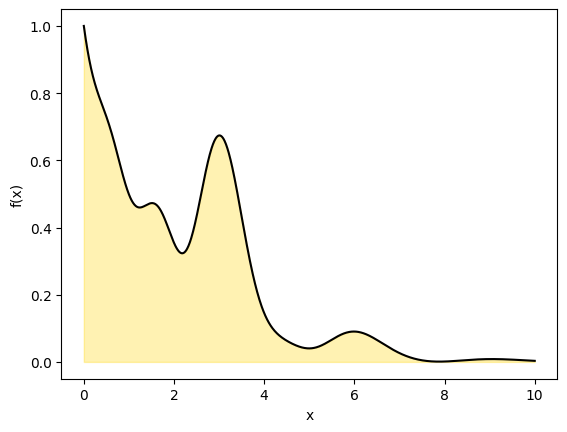
Source
def mc_integral(func,
N=10000,
Lx=2, Ly=1,
plot=True):
'''Generate random points in the square with [0, Lx] and [0, Ly]
Count the fraction of points falling inside the curve
'''
# Generate uniform random numbers
ux = Lx*np.random.rand(N)
uy = Ly*np.random.rand(N)
#Count accepted point.
pinside = uy<func(ux)
# Total area times fraction of sucessful points
I = Lx*Ly*pinside.sum()/N
if plot==True:
plt.plot(ux[pinside], uy[pinside],'o', color='red')
plt.plot(ux[~pinside], uy[~pinside],'o', color='green')
x = np.linspace(0.001, Lx,100)
plt.plot(x, func(x), color='black', lw=2)
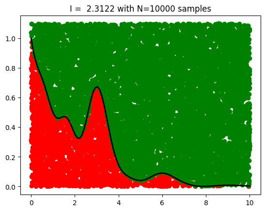
plt.title(f'I = {I:.4f} with N={N} samples',fontsize=12)
return I
### Calculate integral numerically first
from scipy import integrate
#adjust limits of x and y
Lx = 10 # x range from 0 to Lx
Ly = 1.1 # y range from 0 to Ly
y, err = integrate.quad(myfunc1, 0, Lx)
print("Exact result:", y)
I = mc_integral(myfunc1, N=10000, Lx=Lx, Ly=Ly)
print("MC result:", I)Exact result: 2.2898343018663505
MC result: 2.3122
The Essence of Monte Carlo Simulations
Suppose we want to evaluate an integral .
A powerful perspective is to reinterpret this integral as the expectation of a function under some probability distribution :
In this form, the integral becomes the expected value of with respect to the distribution .
To estimate , we draw samples and apply the law of large numbers, which guarantees that the sample average converges to the expected value as :
Simple 1D applications of MC
Ordinary Monte Carlo and Uniform Sampling
A common and intuitive case is when we draw samples uniformly from the interval . In this setting, the sampling distribution is constant: , and the integral simplifies as follows:
This gives a clear interpretation of Monte Carlo integration: we approximate the average height of the function over the interval by randomly sampling points, much like tossing pebbles onto a plot and estimating the shaded area.
Source
x0, x1 = 0, 10
N = 100000
x = np.random.uniform(x0, x1, N)

integral = (x1 - x0) * np.mean(myfunc1(x))

print('MC result', integral)

y, err = integrate.quad(myfunc1, x0, x1)

print("Exact result:", y)
MC result 2.295636864381426
Exact result: 2.2898343018663505
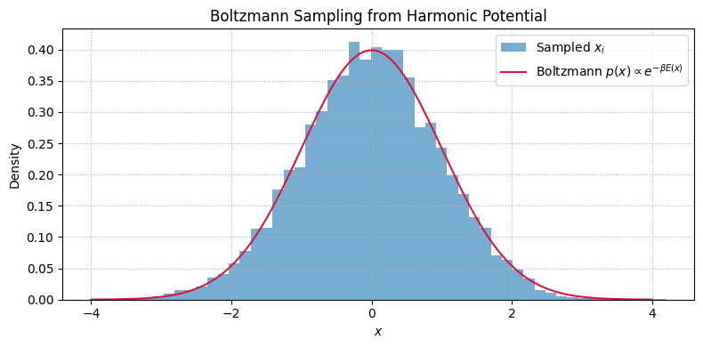
Sampling from the Boltzmann Distribution
Quantities like average energy, heat capacity, or pressure are computed as ensemble averages under the Boltzmann distribution.
The Boltzmann distribution for a system with energy at inverse temperature is:
Suppose we are interested in the average energy:
This is an expectation value under the Boltzmann distribution .
If we can draw samples , we can estimate by:
Source
import numpy as np
import matplotlib.pyplot as plt

# Parameters
beta = 1.0  # inverse temperature
n_samples = 10000

# Boltzmann sampling for harmonic oscillator: Gaussian with variance 1/beta
x_samples = np.random.normal(loc=0.0, scale=np.sqrt(1 / beta), size=n_samples)

# Energy function E(x) = (1/2) * x^2
E = 0.5 * x_samples**2

# Estimate average energy ⟨E⟩
E_mean = np.mean(E)
E_exact = 0.5 / beta

print(f"Estimated ⟨E⟩: {E_mean:.4f}")
print(f"Exact ⟨E⟩:     {E_exact:.4f}")

# Plot histogram and overlay Boltzmann density
x_vals = np.linspace(-4, 4, 500)
p_vals = np.exp(-0.5 * beta * x_vals**2)
p_vals /= np.trapezoid(p_vals, x_vals)  # normalize for display

plt.figure(figsize=(8, 4))
plt.hist(x_samples, bins=50, density=True, alpha=0.6, label='Sampled $x_i$')
plt.plot(x_vals, p_vals, color='crimson', label='Boltzmann $p(x) \\propto e^{-\\beta E(x)}$')
plt.xlabel('$x$')
plt.ylabel('Density')
plt.title('Boltzmann Sampling from Harmonic Potential')
plt.legend()
plt.grid(True, linestyle=':')
plt.tight_layout()
plt.show()
Estimated ⟨E⟩: 0.4924
Exact ⟨E⟩: 0.5000
Source
import numpy as np
from scipy.stats import norm

# Parameters
sigma_x = sigma_y = 1
a = b = 3

# Analytical value of the integral over [-a, a] x [-b, b]
analytical_integral = (norm.cdf(a, scale=sigma_x) - norm.cdf(-a, scale=sigma_x)) * \
                      (norm.cdf(b, scale=sigma_y) - norm.cdf(-b, scale=sigma_y))

# Monte Carlo integration
N = 1_000_000  # Number of samples

# Generate random uniform samples in the rectangle [-a, a] x [-b, b]
x_samples = np.random.uniform(-a, a, N)
y_samples = np.random.uniform(-b, b, N)

# Evaluate the 2D Gaussian at these points
f_values = (1 / (2 * np.pi * sigma_x * sigma_y)) * \
           np.exp(-0.5 * ((x_samples / sigma_x) ** 2 + (y_samples / sigma_y) ** 2))

# Estimate the integral: average value of f * area of the integration region
area = (2 * a) * (2 * b)
monte_carlo_integral = f_values.mean() * area

# Output both results
analytical_integral, monte_carlo_integral
(np.float64(0.9946076967722628), np.float64(0.9960073444788007))MC Integration of a Peaked 2D Function
Let’s visualize how MC integration works on a function with sharp features — a mixture of 2D Gaussians:
This is a good proxy for physical problems where the integrand has localized peaks (e.g., partition functions, reaction coordinates).
Source
import numpy as np
import matplotlib.pyplot as plt
from mpl_toolkits.mplot3d import Axes3D

# ── Define a 2D Gaussian mixture ────────────────────────────────
centers = [(-1.5, -1), (1.5, 1.5), (0, -1.5), (-1, 2)]
sigmas  = [0.4, 0.5, 0.35, 0.45]
weights = [1.0, 0.7, 0.9, 0.6]

def gmm_2d(x, y):
    """2D Gaussian mixture — a peaked, multi-modal function."""
    f = np.zeros_like(x, dtype=float)
    for (cx, cy), s, w in zip(centers, sigmas, weights):
        f += w * np.exp(-((x - cx)**2 + (y - cy)**2) / (2 * s**2))
    return f

# ── Surface grid ───────────────────────────────────────────────
xg = np.linspace(-4, 4, 200)
yg = np.linspace(-4, 4, 200)
X, Y = np.meshgrid(xg, yg)
Z = gmm_2d(X, Y)

# ── MC samples (uniform) ──────────────────────────────────────
N = 5000
xs = np.random.uniform(-4, 4, N)
ys = np.random.uniform(-4, 4, N)
fs = gmm_2d(xs, ys)

# ── Figure: 3D surface + MC samples ───────────────────────────
fig = plt.figure(figsize=(16, 6))

# Left: 3D surface with MC sample points
ax1 = fig.add_subplot(121, projection='3d')
ax1.plot_surface(X, Y, Z, cmap='viridis', alpha=0.7, edgecolor='none')
ax1.scatter(xs[::3], ys[::3], fs[::3], c=fs[::3], cmap='hot', s=4, alpha=0.6)
ax1.set_xlabel('$x$')
ax1.set_ylabel('$y$')
ax1.set_zlabel('$f(x,y)$')
ax1.set_title('MC samples on 2D Gaussian mixture', fontsize=13)
ax1.view_init(elev=30, azim=-45)

# Right: top-down view — contour + scatter colored by f value
ax2 = fig.add_subplot(122)
cont = ax2.contourf(X, Y, Z, levels=30, cmap='viridis', alpha=0.5)
sc = ax2.scatter(xs, ys, c=fs, cmap='hot', s=6, alpha=0.7, edgecolors='none')
plt.colorbar(cont, ax=ax2, label='$f(x,y)$')

# Mark the peaks
for (cx, cy) in centers:
    ax2.plot(cx, cy, 'w*', markersize=12, markeredgecolor='k', markeredgewidth=0.6)

ax2.set_xlabel('$x$', fontsize=13)
ax2.set_ylabel('$y$', fontsize=13)
ax2.set_title('Top view: most uniform samples miss the peaks', fontsize=13)
ax2.set_aspect('equal')

plt.tight_layout()
plt.show()

# ── MC integral estimate ──────────────────────────────────────
area = 8 * 8  # [-4,4] x [-4,4]
I_mc = area * np.mean(fs)
print(f"MC integral estimate (N={N}): {I_mc:.4f}")
print(f"Sample std of f(x_i):         {np.std(fs):.4f}")
print(f"Fraction of samples where f > 0.1: {np.mean(fs > 0.1):.2%}")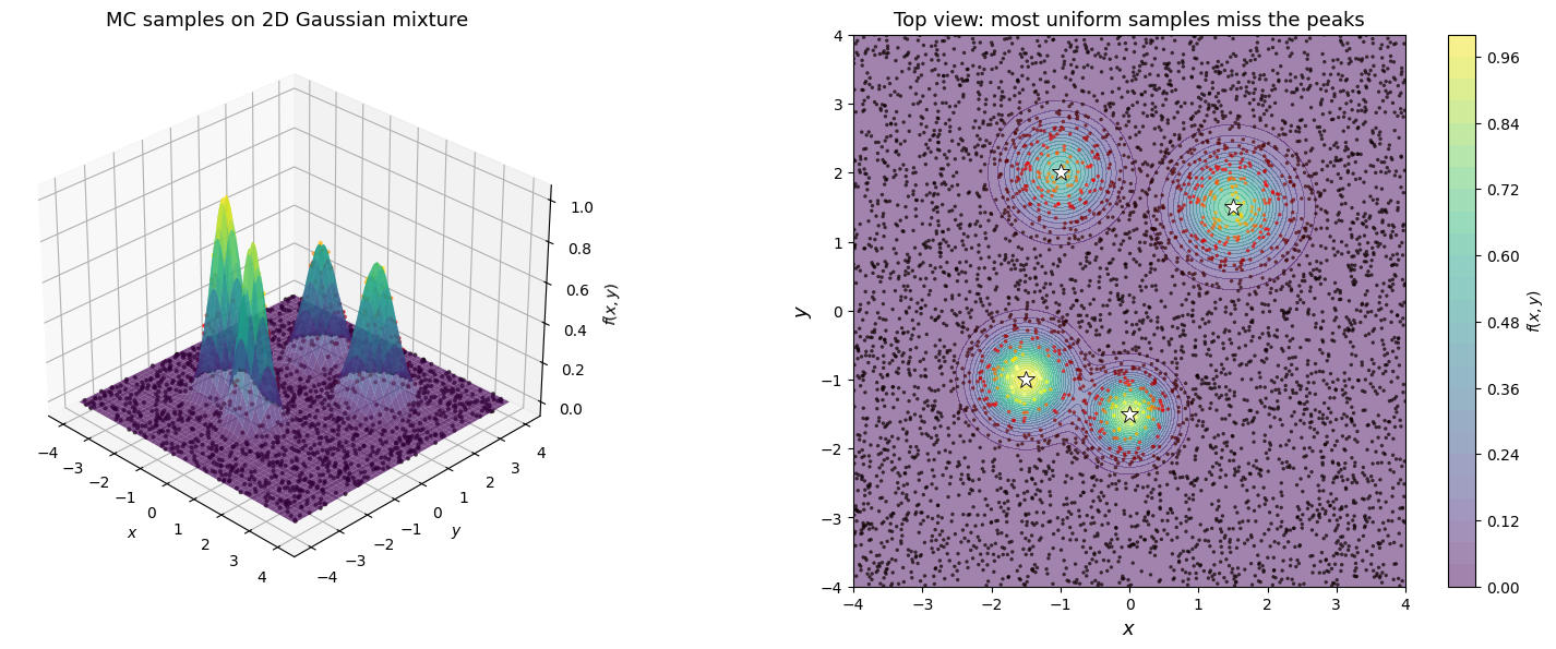
MC integral estimate (N=5000): 3.6243
Sample std of f(x_i):         0.1385
Fraction of samples where f > 0.1: 15.06%
MC vs Grid: the Curse of Dimensionality
The volume of a unit hypersphere in dimensions is .
We can estimate it by MC: throw uniform points in the hypercube, count the fraction inside , and multiply by the cube volume .
As grows, the sphere shrinks relative to the cube — the “hit rate” drops exponentially.
Two ways to do this MC integral — and they behave differently in high :
| Method | Formula | What happens as |
|---|---|---|
| Hit-or-miss | Hit rate , so grows fails | |
| Mean-value | Same formula, convergence rate is still |
The convergence rate is always dimension-independent — that is the superpower of MC over grid methods (which need points).
But itself can grow with when you sample uniformly in a region where the integrand is mostly zero. This does not mean MC is broken — it means uniform sampling is a bad choice of in high dimensions.
This is exactly what motivates importance sampling (choose a smarter ) and eventually MCMC (let the chain find the important regions automatically).
Source
import numpy as np
import matplotlib.pyplot as plt
from scipy.special import gamma

def hypersphere_volume_exact(d):
    """Exact volume of a unit hypersphere in d dimensions."""
    return np.pi**(d / 2) / gamma(d / 2 + 1)

def mc_hypersphere(d, N=500000):
    """MC estimate of the unit hypersphere volume in d dimensions."""
    points = np.random.uniform(-1, 1, size=(N, d))
    inside = np.sum(points**2, axis=1) < 1.0
    hit_rate = np.mean(inside)
    cube_vol = 2**d
    V_mc = cube_vol * hit_rate
    V_err = cube_vol * np.std(inside) / np.sqrt(N)
    return V_mc, V_err, hit_rate

dims = np.arange(2, 16)
V_exact = [hypersphere_volume_exact(d) for d in dims]
V_mc_vals, V_err_vals, hit_rates = zip(*[mc_hypersphere(d) for d in dims])

fig, axes = plt.subplots(1, 3, figsize=(16, 4.5))

# Left: exact vs MC volume
axes[0].semilogy(dims, V_exact, 'ko-', label='Exact $V_d$', lw=2)
axes[0].errorbar(dims, V_mc_vals, yerr=V_err_vals, fmt='s', color='crimson',
                 capsize=4, label='MC estimate')
axes[0].set_xlabel('Dimension $d$', fontsize=13)
axes[0].set_ylabel('Hypersphere volume', fontsize=13)
axes[0].set_title('Volume of unit hypersphere', fontsize=13)
axes[0].legend()
axes[0].grid(True, linestyle=':', alpha=0.5)

# Middle: hit rate (fraction inside sphere)
axes[1].semilogy(dims, hit_rates, 'o-', color='steelblue', lw=2)
axes[1].set_xlabel('Dimension $d$', fontsize=13)
axes[1].set_ylabel('Hit rate (fraction inside)', fontsize=13)
axes[1].set_title('Sphere shrinks relative to cube', fontsize=13)
axes[1].grid(True, linestyle=':', alpha=0.5)

# Right: relative error GROWS with d
rel_err = np.array(V_err_vals) / np.array(V_exact)
axes[2].plot(dims, rel_err * 100, 'o-', color='forestgreen', lw=2)
axes[2].set_xlabel('Dimension $d$', fontsize=13)
axes[2].set_ylabel('Relative error (%)', fontsize=13)
axes[2].set_title(r'Relative error grows: $\sigma$ grows with $d$', fontsize=13)
axes[2].grid(True, linestyle=':', alpha=0.5)

plt.suptitle('Uniform MC integration across dimensions (N=500k)', fontsize=15, y=1.02)
plt.tight_layout()
plt.show()

print(f"\nAt d=2:  hit rate = {hit_rates[0]:.3f},  relative error = {rel_err[0]*100:.1f}%")
print(f"At d=15: hit rate = {hit_rates[-1]:.5f},  relative error = {rel_err[-1]*100:.1f}%")
print(f"\nThe rate is always O(1/sqrt(N)), but sigma grows => need smarter sampling!")
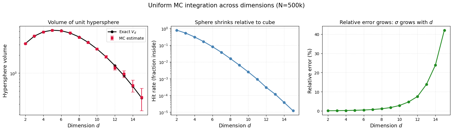
At d=2:  hit rate = 0.785,  relative error = 0.1%
At d=15: hit rate = 0.00001,  relative error = 42.1%

The rate is always O(1/sqrt(N)), but sigma grows => need smarter sampling!
Why Does Monte Carlo Outperform Brute-Force Integration?
By the Central Limit Theorem, the sample mean has variance that decreases with the number of samples:
where is the variance of a single sample. This gives a standard error of .
Consequently, the convergence rate of Monte Carlo integration is , independent of the number of dimensions.
By contrast, deterministic grid-based quadrature methods in dimensions have a convergence rate of , where is the order of the method. This means they slow down exponentially as dimensionality grows — the curse of dimensionality.
Even in low-dimensional scenarios, Monte Carlo can be advantageous when the region of significant contribution within the integration space is small, allowing for targeted sampling in critical areas.
On convergence of MC simulations
We are often interested in knowing how many iterations it takes for Monte Carlo integration to “converge”. To do this, we would like some estimate of the variance, and it is useful to inspect such plots. One simple way to get confidence intervals for the plot of Monte Carlo estimate against number of iterations is simply to do many such simulations.
For the example, we will try to estimate the function (again)
Source
def f(x):
    return x * np.cos(71*x) + np.sin(13*x)

x = np.linspace(0, 1, 100)

plt.plot(x, f(x),linewidth=2.0)


plt.xlabel(r'$x$',fontsize=20)
plt.ylabel(r'$f(x)$',fontsize=20)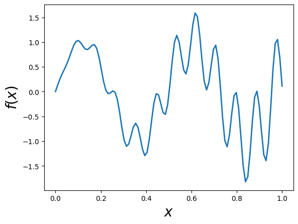
We will vary the sample size from 1 to 100 and calculate the value of for 1000 replicates. We then plot the 2.5th and 97.5th percentile of the 1000 values of to see how the variation in changes with sample size.
Source
n = 100
reps = 1000

# Generating random numbers and applying the function
fx = f(np.random.random((n, reps)))

# Calculating cumulative mean for each simulation
y = np.cumsum(fx, axis=0) / np.arange(1, n+1)[:, None]

# Calculating the upper and lower percentiles
upper, lower = np.percentile(y, [97.5, 2.5], axis=1)

# Plotting the results
plt.figure(figsize=(10, 6))
for i in range(reps):
    plt.plot(np.arange(1, n+1), y[:, i], c='grey', alpha=0.02)
plt.plot(np.arange(1, n+1), y[:, 0], c='red', linewidth=1)
plt.plot(np.arange(1, n+1), upper, 'b', label='97.5th percentile')
plt.plot(np.arange(1, n+1), lower, 'b', label='2.5th percentile')

plt.xlabel('Number of independent MC runs')
plt.ylabel('Cumulative mean of f(x)')
plt.title('Monte Carlo Simulations')
plt.legend()
plt.show()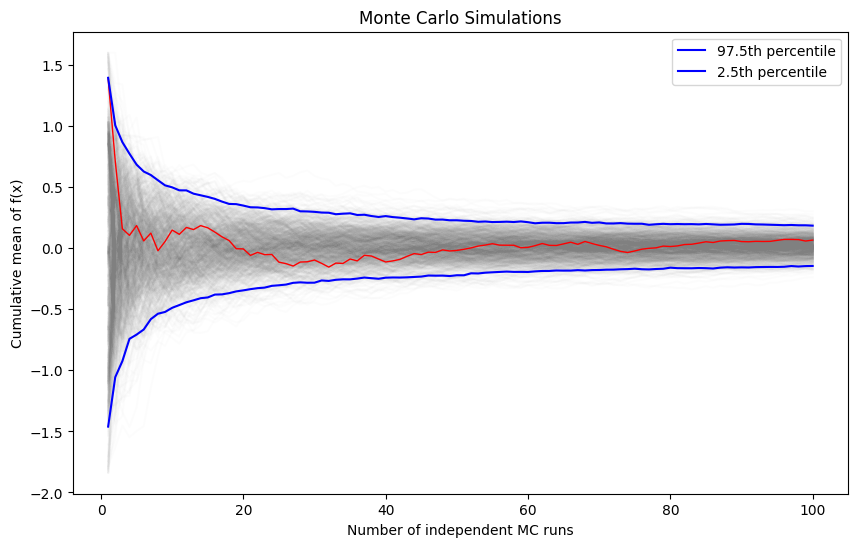
Two knobs for reducing MC error: more samples vs smarter sampling
The MC error is always . There are two independent knobs to reduce it:
| Knob | What it does | How |
|---|---|---|
| Increase | Shrink | Throw more samples (brute force) |
| Decrease | Shrink the prefactor | Sample where the integrand matters (importance sampling) |
When uniform sampling fails: If is sharply peaked (e.g., a Boltzmann factor at low ), most uniform samples land where . A few rare samples hit the peak and return huge values. This makes enormous — so even though shrinks with , you’re starting from a huge .
Importance sampling attacks the directly: by sampling from a distribution that concentrates points where is large, the reweighted values become nearly constant across samples, dramatically reducing variance.
Importance Sampling
Suppose we want to evaluate the expectation of a function under a probability distribution :
If sampling directly from is difficult, we can instead introduce an alternative distribution — one that is easier to sample from — and rewrite the integral as:
This reformulation allows us to draw samples , and weight them by the importance ratio . The expectation can then be estimated using:
This is the essence of importance sampling: reweighting samples from an easier distribution to approximate expectations under a more complex one.
Source
import numpy as np
import matplotlib.pyplot as plt
import matplotlib as mpl
# Define the unnormalized target distribution: p(y) ∝ exp(-y^4 + y^2)
def p(y):
return np.exp(-y**4 + y**2)
# Uniform proposal over [a, b]
a, b = -5, 5
def q_uniform(y):
return np.ones_like(y) / (b - a)
# Gaussian proposal centered at mode of p(y)
mu_q_better = 0.0
sigma_q_better = 1.0
def q_better(y):
return (1 / (np.sqrt(2 * np.pi) * sigma_q_better)) * np.exp(-(y - mu_q_better)**2 / (2 * sigma_q_better**2))
# Dense sampling sizes for smoother convergence curves
sample_sizes = np.logspace(2, 4.5, num=20, dtype=int) # From 100 to ~30,000
# Store estimates
uniform_estimates = []
better_estimates = []
# Estimate normalizing constant Z = ∫ p(y) dy
for N in sample_sizes:
# Uniform proposal
y_uniform = np.random.uniform(low=a, high=b, size=N)
weights_uniform = p(y_uniform) / q_uniform(y_uniform)
uniform_estimates.append(np.mean(weights_uniform))
# Better Gaussian proposal
y_better = np.random.normal(loc=mu_q_better, scale=sigma_q_better, size=N)
weights_better = p(y_better) / q_better(y_better)
better_estimates.append(np.mean(weights_better))
# Plotting
plt.figure(figsize=(10, 6))
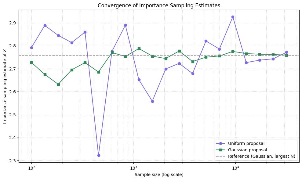
plt.plot(sample_sizes, uniform_estimates, label='Uniform proposal', color='mediumslateblue', marker='o')
plt.plot(sample_sizes, better_estimates, label='Gaussian proposal', color='seagreen', marker='s')
plt.axhline(y=better_estimates[-1], linestyle='--', color='gray', label='Reference (Gaussian, largest N)')
plt.xscale('log')
plt.xlabel('Sample size (log scale)')
plt.ylabel('Importance sampling estimate of Z')
plt.title('Convergence of Importance Sampling Estimates')
plt.grid(True, which='both', linestyle=':', alpha=0.7)
plt.legend()
plt.tight_layout()
plt.show()
Source
# Range for plotting
y_vals = np.linspace(-6, 6, 1000)

# Evaluate functions
p_vals = p(y_vals)

# Determine region of significant mass: where p(y) > 1% of max
threshold = 0.01 * np.max(p_vals)
mask = p_vals > threshold
y_zoom = y_vals[mask]
p_zoom = p_vals[mask]
q_uniform_zoom = q_uniform(y_zoom)
q_better_zoom = q_better(y_zoom)

# Normalize p for plotting
p_zoom_normalized = p_zoom / np.trapezoid(p_zoom, y_zoom)

# Importance weights (unnormalized)
w_uniform_zoom = p_zoom / q_uniform_zoom
w_better_zoom = p_zoom / q_better_zoom

# Plot
fig, axes = plt.subplots(2, 1, figsize=(10, 10), sharex=True)

# Top: Distributions
axes[0].plot(y_zoom, p_zoom_normalized, label='Target $p(y)$ (normalized)', color='crimson', linewidth=2)
axes[0].plot(y_zoom, q_uniform_zoom, label='Uniform proposal $q_{\\mathrm{uniform}}$', color='dodgerblue', linestyle='--')
axes[0].plot(y_zoom, q_better_zoom, label='Gaussian proposal $q_{\\mathrm{better}}$', color='forestgreen', linestyle='-.')
axes[0].set_ylabel('Density')
axes[0].set_title('Zoomed-In Target and Proposal Distributions')
axes[0].legend()
axes[0].grid(True, linestyle=':', alpha=0.7)

# Bottom: Weights
axes[1].plot(y_zoom, w_uniform_zoom, label=r'$w(y) = p(y)/q_{\mathrm{uniform}}$', color='dodgerblue', linestyle='--')
axes[1].plot(y_zoom, w_better_zoom, label=r'$w(y) = p(y)/q_{\mathrm{better}}$', color='forestgreen', linestyle='-.')
axes[1].set_xlabel('$y$')
axes[1].set_ylabel('Importance weight')
axes[1].set_yscale('log')
axes[1].set_title('Zoomed-In Importance Weights (Log Scale)')
axes[1].legend()
axes[1].grid(True, linestyle=':', alpha=0.7)

plt.tight_layout()
plt.show()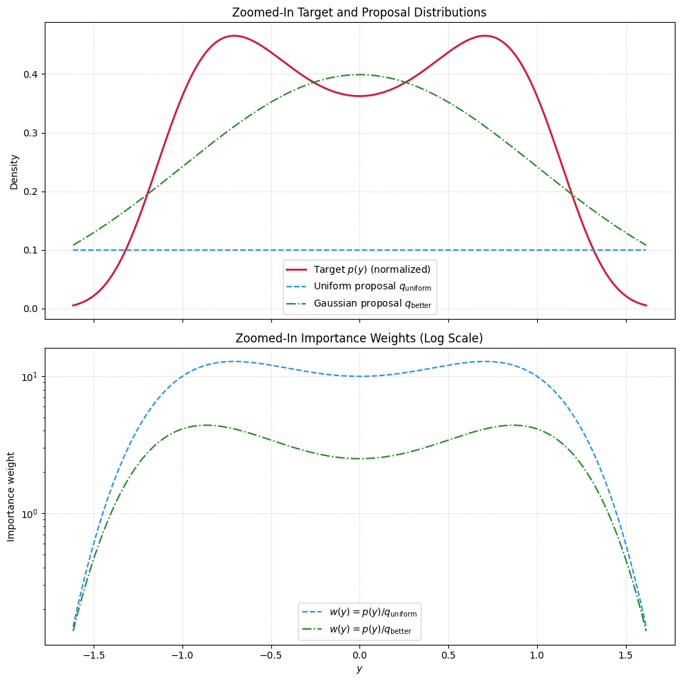
Using Monte Carlo to sample probability distributions
Another application of a simple MC technique is to turn uniformly distributed random numbers into random numbers sampled according to different probability distributions.
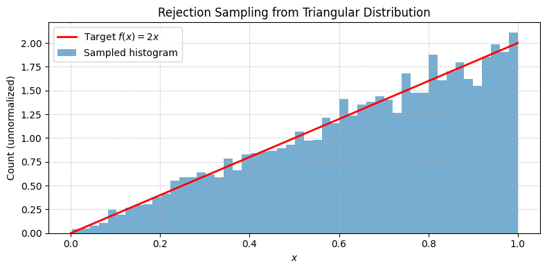
The key is to employ rejection criteria; if points go under the curve, they are accepted, hence generating a probability distribution
Source
import numpy as np
import matplotlib.pyplot as plt

# Target unnormalized PDF: f(x) = 2x on [0, 1]
f = lambda x: 2 * x
Lx, Ly, N = 1, 2, 10000  # Domain, max height, number of samples

# Rejection sampling
x = Lx * np.random.rand(N)
y = Ly * np.random.rand(N)
accepted = x[y <= f(x)]

# Plot result
x_plot = np.linspace(0, 1, 500)
plt.figure(figsize=(8, 4))
plt.plot(x_plot, f(x_plot), 'r-', lw=2, label='Target $f(x) = 2x$')
plt.hist(accepted, bins=50, alpha=0.6, density=True, label='Sampled histogram')
plt.title('Rejection Sampling from Triangular Distribution')
plt.xlabel('$x$')
plt.ylabel('Count (unnormalized)')
plt.legend()
plt.grid(True, linestyle=':')
plt.tight_layout()
plt.show()
Problems
MC, the crude version
Evaluate the following integral using Monte Carlo methods.
Start by doing a direct monte carlo on uniform interval.
Try an importance sampling approach using en exponential probability distribution.
Find the optimal value of that gives the most rapid reduction of variance [Hint: experiment with different values of ]
MC integral of 3D and 6D spheres!
Generalize the MC code above for computing the volume of 3D and 6D spheres.
The analytical results are known: and . So you can check the statistical error made in the simulations.