Phases, phase diagrams, and phase transitions
A phase is a macroscopic state of matter characterized by uniform physical properties: density, magnetization, crystal structure, etc. A phase diagram maps out which phase is stable as a function of thermodynamic variables like temperature and pressure.
Phase transitions occur when the system crosses a phase boundary. But not every path through the diagram encounters one:
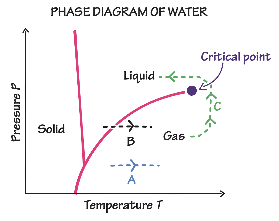
Phase diagram for fluids. Path A stays within a single phase — no transition. Path B crosses the coexistence line and undergoes an abrupt phase transition. Path C circumvents the critical point, so the change is gradual and continuous.
A brief history of phase transitions
1895 — Pierre Curie studies magnetism in his doctoral thesis and discovers:
Magnetic properties change dramatically with temperature
A sharp phase transition occurs at what is now called the Curie point
The phenomenon has its origin at the atomic scale
Timeline: from Lenz to the renormalization group
1920 — Lenz proposes a lattice model for ferromagnetism, arguing that atomic dipoles occupy one of two orientations. He assigns the problem to his PhD student.
1924 — Ernst Ising solves the one-dimensional version exactly and finds no phase transition. He incorrectly concludes that no transition occurs in any dimension, and leaves academic research. Despite this, the paper attracts attention from Pauli, Heisenberg, and Dirac.
1936 — Rudolf Peierls proves that the 2D model does undergo a finite-temperature phase transition, revitalizing interest and demonstrating the crucial role of dimensionality.
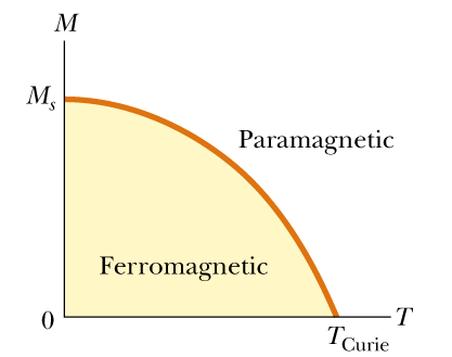
Spontaneous magnetization in a ferromagnet: a continuous phase transition from ordered to disordered phase with increasing temperature.
1941 — Kramers and Wannier calculate the critical temperature of the 2D model using a duality argument.
1944 — Lars Onsager solves the 2D Ising model exactly — a landmark of theoretical physics. Exact expressions for the partition function, free energy, and magnetization follow. Onsager, trained as a chemist, was part of a tradition of chemists (later including Ben Widom) who made foundational contributions to phase transition theory.
1944 onward — The Ising model becomes a canonical testing ground for new mathematical techniques: transfer matrices, cluster expansions, combinatorics, and series methods. Applications spread to biology, chemistry, economics, and computer science.
1970s — Kenneth Wilson develops the renormalization group (Nobel Prize, 1982). Key insights: the critical point is universal (translation-, scale-, and rotation-invariant), and coarse-graining explains why microscopically different systems share the same critical behavior.
1985 — Conformal Field Theory (CFT) provides an elegant framework for 2D critical systems, linking statistical mechanics and quantum field theory through symmetry principles.
The Ising Model: the hydrogen atom of phase transitions
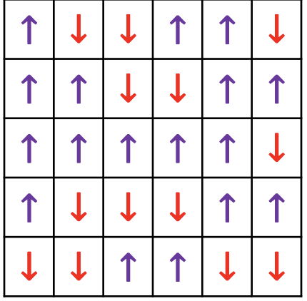
The Ising model: each lattice site carries a spin that points either up (+1) or down (-1).
What do Ising configurations look like?
Before diving into simulations, let’s build visual intuition. The plots below show random spin configurations with increasing alignment bias — from a fully disordered state (high ) to a nearly ordered state (low ). In reality, the degree of ordering is set self-consistently by the Boltzmann distribution, but even this simple exercise reveals the visual hallmark of a phase transition: a change from a disordered “salt-and-pepper” pattern to large uniform domains.
Source
import numpy as np
import matplotlib.pyplot as plt

fig, axes = plt.subplots(1, 4, figsize=(14, 3.5))

biases = [0.5, 0.65, 0.85, 0.98]
labels = ['Disordered\n($T \gg T_c$)', 'Weakly ordered', 'Partially ordered', 'Strongly ordered\n($T \ll T_c$)']
N = 40

for ax, p_up, label in zip(axes, biases, labels):
    spins = np.random.choice([-1, 1], size=(N, N), p=[1 - p_up, p_up])
    ax.imshow(spins, cmap='coolwarm', vmin=-1, vmax=1, interpolation='nearest')
    ax.set_title(label, fontsize=11)
    ax.set_xticks([])
    ax.set_yticks([])

fig.suptitle('Random spin configurations with increasing alignment bias', fontsize=13, y=1.02)
plt.tight_layout()
plt.show()
First-order vs continuous phase transitions
Phase transitions come in two fundamentally different kinds:
First-order transitions involve a discontinuous jump in an order parameter (e.g., density in liquid-gas, magnetization under a field). The system releases or absorbs latent heat, and the two phases coexist at the transition. Example: ice melting to water at 0 °C.
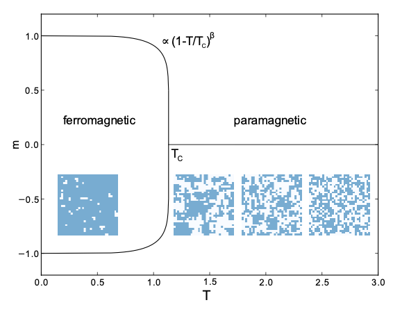
Continuous (second-order) transitions show no discontinuity in the order parameter itself, but its derivatives (susceptibility, heat capacity) diverge. There is no latent heat and no phase coexistence. Example: the ferromagnetic-to-paramagnetic transition at the Curie temperature.
-c1976648826bc3fe1472e5a554a040a1.png)
Left: first-order transition with a discontinuous jump in the order parameter. Right: continuous transition where the order parameter vanishes smoothly.
Critical phenomena: diverging correlation length
Near a continuous phase transition, the correlation length — the typical distance over which spins “know about” each other — grows without bound. At , the system becomes scale-invariant: fluctuations of all sizes coexist, and there is no characteristic length scale left in the problem.
This divergence of is the root cause of all critical phenomena: it is why response functions (, ) diverge, why critical slowing down occurs in dynamics, and why the system looks statistically self-similar at every scale.
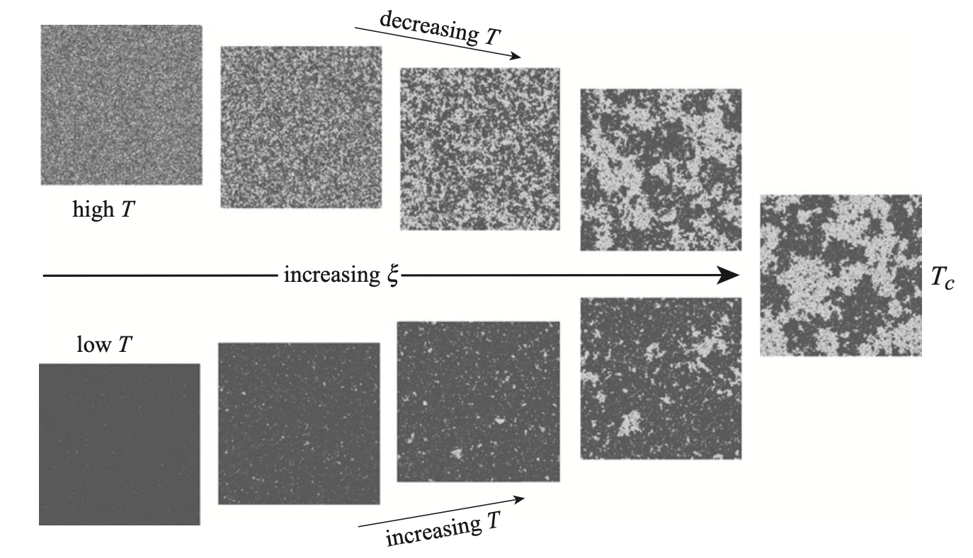
As , the correlation length diverges. Spin clusters grow to span the entire system.
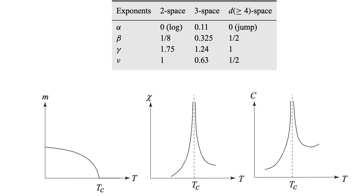
Critical exponents and scaling
Near , thermodynamic quantities obey power laws characterized by critical exponents:
| Quantity | Symbol | Power law | Exponent |
|---|---|---|---|
| Order parameter | |||
| Susceptibility | $\chi \sim | T - T_c | |
| Heat capacity | $C_V \sim | T - T_c | |
| Correlation length | $\xi \sim | T - T_c |
These exponents are not independent — they are connected by scaling relations such as the Rushbrooke inequality and the hyperscaling relation (where is the spatial dimension).
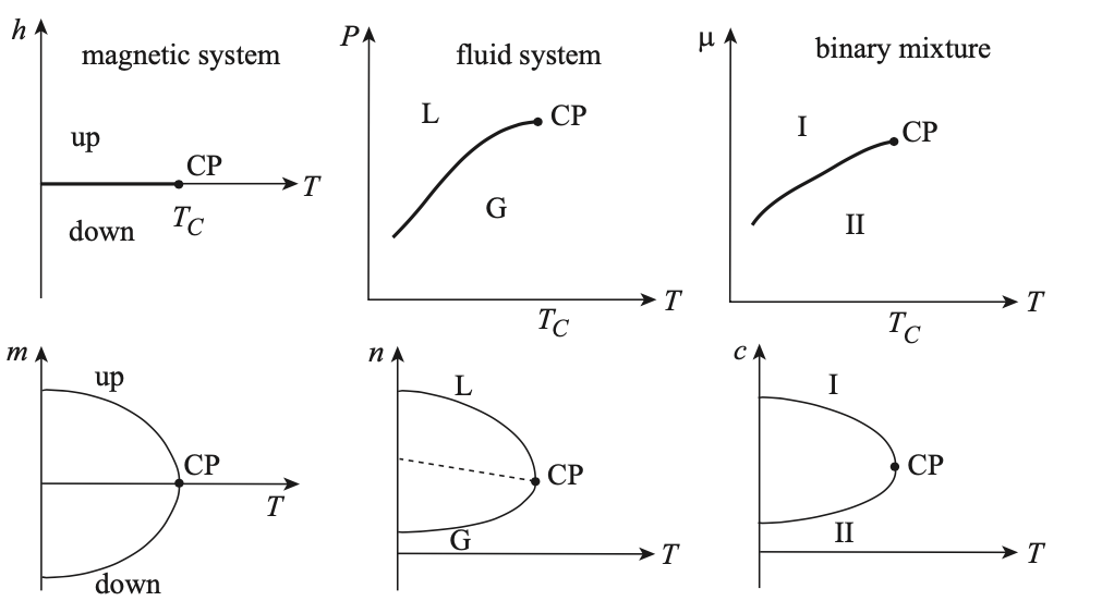
Universality
The most remarkable feature of critical phenomena is universality: systems with completely different microscopic physics share the same critical exponents if they have the same:
Spatial dimensionality
Symmetry of the order parameter (e.g., scalar vs vector)
Range of interactions (short- vs long-range)
This is why the liquid-gas critical point, the Curie point in ferromagnets, and the demixing transition in binary fluids all fall into the same universality class. The renormalization group explains this: near the correlation length , and microscopic details are averaged away, leaving only symmetry and dimensionality.
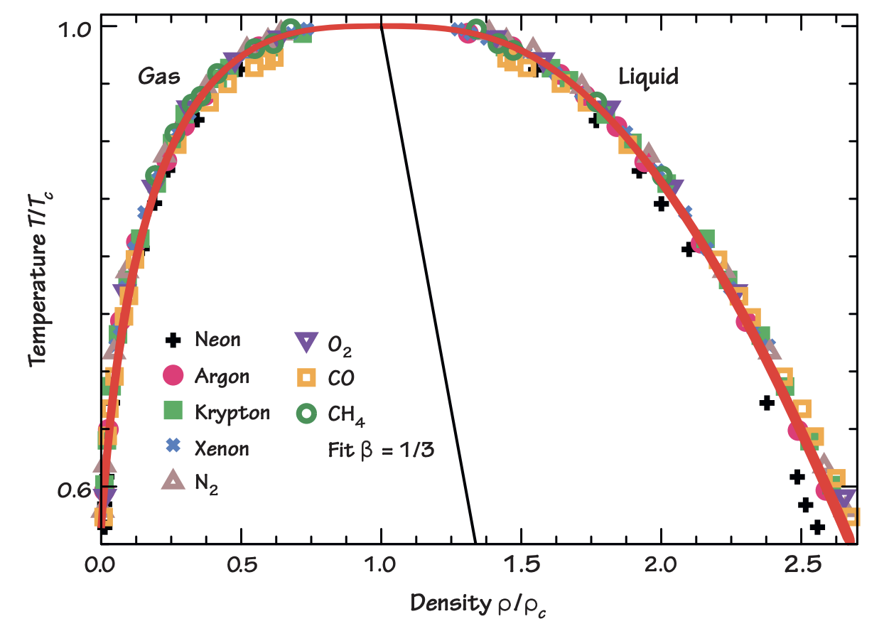
Universality in fluids: different substances collapse onto the same curve when plotted in reduced variables.
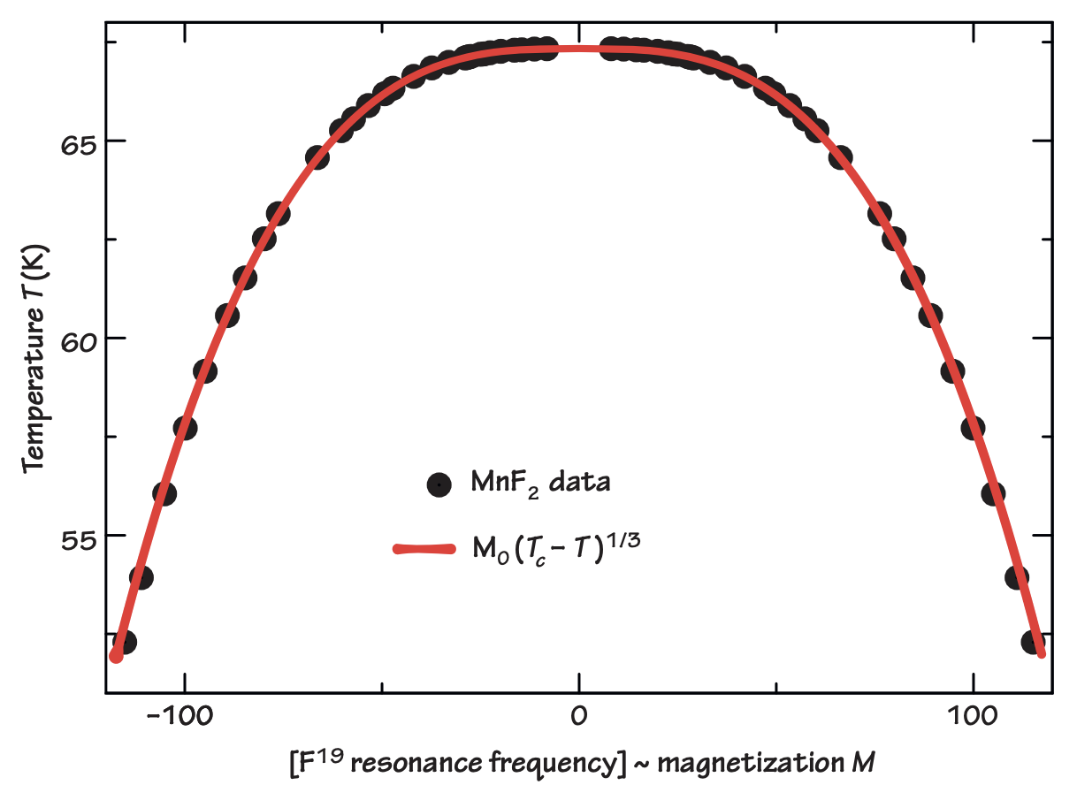
Universality in magnetic systems: different ferromagnets share the same critical exponents.
Thermodynamics of magnetic systems
For a magnetic system in an external field , the fundamental thermodynamic relation acquires a magnetic work term:
Performing a Legendre transform to obtain the Helmholtz free energy :
This gives us direct access to magnetization and entropy as derivatives of :
Fluctuations, correlations, and response functions
The connection between microscopic fluctuations and macroscopic response is a central theme of statistical mechanics. For the Ising model, three quantities play a key role:
Heat capacity measures energy fluctuations:
Magnetic susceptibility measures magnetization fluctuations:
Correlation function quantifies how strongly two spins influence each other:
At high temperature, spins are nearly independent and decays rapidly with distance. At low temperature, spins are strongly correlated over large distances. The correlation length characterizes the decay: . At the critical point, and correlations become long-ranged.
Applications of the Ising model beyond magnetism
The Ising model’s power lies in its generality — any system of binary variables with local interactions maps onto it:
Ferromagnetism. The Ising model is the scalar () special case of the more general Heisenberg model with vector spins.
Binary alloys and lattice gases. Each site is occupied by atom A () or B (). Nearest-neighbor interaction energies , , map to an effective coupling . The Ising model thus describes order-disorder transitions in alloy composition.
Spin glasses. Each bond gets its own coupling drawn from a random distribution, mixing ferromagnetic and antiferromagnetic interactions. This models structurally disordered systems with competing interactions.
Biomolecular conformations. The helix-coil transition in DNA: means a hydrogen bond is closed, means it is open. The transition between helix and coil is an Ising-like phase transition. Other examples include oxygen-binding cooperativity in hemoglobin and conformational switching in bacterial flagella.
Neural networks. In the Hopfield model, means a neuron is firing and means it is resting. Boltzmann machines — used in machine learning — are a stochastic generalization of this idea.
Epidemics and opinion dynamics. In models of disease or rumor spreading, means “infected” and means “susceptible.” If nearest-neighbor coupling is strong enough, a macroscopic fraction of the population becomes infected — a phase transition.
The Peierls Argument
In the 1930s, Rudolf Peierls devised an elegant scaling argument that explains why the Ising model has a phase transition in 2D but not in 1D. The key idea is to compare the energy cost of creating a domain of flipped spins against the entropy gain from the number of ways to place it.
No phase transition in 1D at 
Start with a 1D chain of spins, all pointing up. Now create a domain of flipped spins by introducing two domain walls:
Energy cost. Each domain wall breaks one nearest-neighbor bond at a cost of . Two walls cost:
Entropy gain. The two walls can be placed at any of pairs of positions along the chain:
Free energy change:
For any finite and , : it is always favorable to create domain walls. Entropy wins at every temperature, destroying long-range order. There is no phase transition in 1D at finite temperature.
Phase transition in 2D at 
In 2D, a domain of flipped spins is bounded by a closed contour of length — a macroscopic quantity, unlike the fixed cost of two point-like walls in 1D.
Energy cost. Each bond along the contour costs :
Entropy gain. The number of self-avoiding contours of length on a square lattice grows roughly as (at each step, the contour can go in directions):
Free energy change:
At low temperatures, : creating a domain boundary is costly and the ordered phase is stable. Domain walls become favorable only when:
This is a rough estimate (the exact Onsager result is ), but the essential physics is captured: in 2D, the energy cost of a domain wall grows with its size, and a finite critical temperature exists.
Exact solution of the 1D Ising model (transfer matrix)
The 1D Ising model with periodic boundary conditions can be solved exactly using the transfer matrix method. For spins in a ring with coupling and external field , the partition function is:
where is the transfer matrix with eigenvalues:
In the thermodynamic limit (), only the largest eigenvalue matters: . Since is analytic for all finite , the free energy has no singularity — confirming that no phase transition occurs in 1D.
Source
import numpy as np
import matplotlib.pyplot as plt

def ising_1d_exact(T_range, J=1.0, h=0.0):
    """Exact thermodynamics of the 1D Ising model via transfer matrix."""
    E_list, M_list, Cv_list, chi_list = [], [], [], []

    for T in T_range:
        beta = 1.0 / T

        # Transfer matrix eigenvalues
        lam_p = np.exp(beta * J) * np.cosh(beta * h) + np.sqrt(
            np.exp(2 * beta * J) * np.sinh(beta * h)**2 + np.exp(-2 * beta * J))

        # Free energy per spin
        def log_lam_plus(b):
            return np.log(np.exp(b * J) * np.cosh(b * h) + np.sqrt(
                np.exp(2 * b * J) * np.sinh(b * h)**2 + np.exp(-2 * b * J)))

        def free_energy(TT):
            return -TT * log_lam_plus(1.0 / TT)

        def free_energy_h(hh):
            bb = beta
            return -T * np.log(np.exp(bb * J) * np.cosh(bb * hh) + np.sqrt(
                np.exp(2 * bb * J) * np.sinh(bb * hh)**2 + np.exp(-2 * bb * J)))

        # Numerical derivatives
        dT = T * 1e-5
        dbeta = beta * 1e-5
        dh = 1e-5

        E = -(log_lam_plus(beta + dbeta) - log_lam_plus(beta - dbeta)) / (2 * dbeta)
        Cv = -(free_energy(T + dT) - 2 * free_energy(T) + free_energy(T - dT)) / (dT**2) / T
        M = -(free_energy_h(h + dh) - free_energy_h(h - dh)) / (2 * dh)
        chi = -(free_energy_h(h + dh) - 2 * free_energy_h(h) + free_energy_h(h - dh)) / (dh**2)

        E_list.append(E)
        M_list.append(abs(M))
        Cv_list.append(Cv)
        chi_list.append(chi)

    return np.array(E_list), np.array(M_list), np.array(Cv_list), np.array(chi_list)

T = np.linspace(0.1, 5.0, 200)
E, M, Cv, chi = ising_1d_exact(T, J=1.0, h=0.0)

fig, axes = plt.subplots(2, 2, figsize=(10, 7))

axes[0, 0].plot(T, E, color='steelblue', lw=2)
axes[0, 0].set(ylabel='$\\langle E \\rangle / N$', xlabel='$T \; [J/k_B]$')

axes[0, 1].plot(T, M, color='crimson', lw=2)
axes[0, 1].set(ylabel='$\\langle |M| \\rangle / N$', xlabel='$T \; [J/k_B]$')

axes[1, 0].plot(T, Cv, color='darkorange', lw=2)
axes[1, 0].set(ylabel='$C_V / N k_B$', xlabel='$T \; [J/k_B]$')

axes[1, 1].plot(T, chi, color='seagreen', lw=2)
axes[1, 1].set(ylabel='$\\chi / N$', xlabel='$T \; [J/k_B]$')

fig.suptitle('Exact 1D Ising model ($h = 0$): no phase transition at finite $T$', fontsize=13)
plt.tight_layout()
plt.show()
<>:51: SyntaxWarning: invalid escape sequence '\;'
<>:54: SyntaxWarning: invalid escape sequence '\;'
<>:57: SyntaxWarning: invalid escape sequence '\;'
<>:60: SyntaxWarning: invalid escape sequence '\;'
<>:51: SyntaxWarning: invalid escape sequence '\;'
<>:54: SyntaxWarning: invalid escape sequence '\;'
<>:57: SyntaxWarning: invalid escape sequence '\;'
<>:60: SyntaxWarning: invalid escape sequence '\;'
/var/folders/77/92dtv6bs0gn66v7t347kmd_w0000gp/T/ipykernel_35738/1365231200.py:51: SyntaxWarning: invalid escape sequence '\;'
axes[0, 0].set(ylabel='$\\langle E \\rangle / N$', xlabel='$T \; [J/k_B]$')
/var/folders/77/92dtv6bs0gn66v7t347kmd_w0000gp/T/ipykernel_35738/1365231200.py:54: SyntaxWarning: invalid escape sequence '\;'
axes[0, 1].set(ylabel='$\\langle |M| \\rangle / N$', xlabel='$T \; [J/k_B]$')
/var/folders/77/92dtv6bs0gn66v7t347kmd_w0000gp/T/ipykernel_35738/1365231200.py:57: SyntaxWarning: invalid escape sequence '\;'
axes[1, 0].set(ylabel='$C_V / N k_B$', xlabel='$T \; [J/k_B]$')
/var/folders/77/92dtv6bs0gn66v7t347kmd_w0000gp/T/ipykernel_35738/1365231200.py:60: SyntaxWarning: invalid escape sequence '\;'
axes[1, 1].set(ylabel='$\\chi / N$', xlabel='$T \; [J/k_B]$')
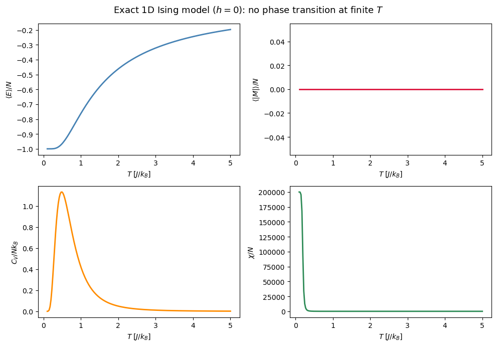
The 1D results confirm the Peierls argument: energy and magnetization change smoothly — there is no singularity, no divergence in or , and no spontaneous magnetization at any . The heat capacity shows a broad Schottky-like peak rather than a sharp divergence.
Exact enumeration of a small 2D Ising lattice
For small enough lattices, we can enumerate every microstate and compute the partition function exactly. A lattice has states — perfectly tractable.
This brute-force approach gives us exact thermodynamic averages and reveals the signatures of the 2D phase transition: a peak in and near , and a smooth crossover in and . Compare the sharp features here with the smooth 1D curves above.
Source
import numpy as np
import matplotlib.pyplot as plt
from itertools import product

def exact_ising_2d(L, J=1.0, h=0.0, T_range=np.linspace(0.5, 5.0, 60)):
    """Exact enumeration of all 2^(L*L) states for an L x L Ising model with PBC."""
    N = L * L
    sites = list(product([-1, 1], repeat=N))

    # Precompute neighbor pairs (right and down, with periodic boundaries)
    neighbors = []
    for i in range(L):
        for j in range(L):
            idx = i * L + j
            right = i * L + (j + 1) % L
            down = ((i + 1) % L) * L + j
            neighbors.append((idx, right))
            neighbors.append((idx, down))

    # Energy and magnetization for every microstate
    energies = np.zeros(len(sites))
    mags = np.zeros(len(sites))
    for k, state in enumerate(sites):
        s = np.array(state)
        E = 0.0
        for (a, b) in neighbors:
            E -= J * s[a] * s[b]
        E -= h * np.sum(s)
        energies[k] = E
        mags[k] = np.sum(s)

    # Thermodynamic averages at each temperature
    results = {'T': T_range, 'E': [], 'M': [], 'Cv': [], 'chi': []}
    for T in T_range:
        beta = 1.0 / T
        logw = -beta * energies
        logw -= logw.max()
        w = np.exp(logw)
        Z = w.sum()
        p = w / Z

        E_avg = np.dot(p, energies) / N
        E2_avg = np.dot(p, energies**2) / N**2
        M_avg = np.dot(p, np.abs(mags)) / N
        M2_avg = np.dot(p, mags**2) / N**2

        results['E'].append(E_avg)
        results['M'].append(M_avg)
        results['Cv'].append((E2_avg - (np.dot(p, energies) / N)**2) / T**2)
        results['chi'].append((M2_avg - M_avg**2) / T)

    return results

res = exact_ising_2d(L=4)
Tc_onsager = 2.0 / np.log(1 + np.sqrt(2))

fig, axes = plt.subplots(2, 2, figsize=(10, 7))

axes[0, 0].plot(res['T'], res['E'], 'o-', color='steelblue', ms=3)
axes[0, 0].axvline(Tc_onsager, ls='--', color='gray', alpha=0.7, label=f'$T_c$ (Onsager) = {Tc_onsager:.3f}')
axes[0, 0].set(ylabel='$\\langle E \\rangle / N$', xlabel='$T \; [J/k_B]$')
axes[0, 0].legend(fontsize=9)

axes[0, 1].plot(res['T'], res['M'], 'o-', color='crimson', ms=3)
axes[0, 1].axvline(Tc_onsager, ls='--', color='gray', alpha=0.7)
axes[0, 1].set(ylabel='$\\langle |M| \\rangle / N$', xlabel='$T \; [J/k_B]$')

axes[1, 0].plot(res['T'], res['Cv'], 'o-', color='darkorange', ms=3)
axes[1, 0].axvline(Tc_onsager, ls='--', color='gray', alpha=0.7)
axes[1, 0].set(ylabel='$C_V / N k_B$', xlabel='$T \; [J/k_B]$')

axes[1, 1].plot(res['T'], res['chi'], 'o-', color='seagreen', ms=3)
axes[1, 1].axvline(Tc_onsager, ls='--', color='gray', alpha=0.7)
axes[1, 1].set(ylabel='$\\chi / N$', xlabel='$T \; [J/k_B]$')

fig.suptitle('Exact enumeration: $4 \\times 4$ Ising model ($h = 0$)', fontsize=13)
plt.tight_layout()
plt.show()
<>:61: SyntaxWarning: invalid escape sequence '\;'
<>:66: SyntaxWarning: invalid escape sequence '\;'
<>:70: SyntaxWarning: invalid escape sequence '\;'
<>:74: SyntaxWarning: invalid escape sequence '\;'
<>:61: SyntaxWarning: invalid escape sequence '\;'
<>:66: SyntaxWarning: invalid escape sequence '\;'
<>:70: SyntaxWarning: invalid escape sequence '\;'
<>:74: SyntaxWarning: invalid escape sequence '\;'
/var/folders/77/92dtv6bs0gn66v7t347kmd_w0000gp/T/ipykernel_35738/3285649429.py:61: SyntaxWarning: invalid escape sequence '\;'
axes[0, 0].set(ylabel='$\\langle E \\rangle / N$', xlabel='$T \; [J/k_B]$')
/var/folders/77/92dtv6bs0gn66v7t347kmd_w0000gp/T/ipykernel_35738/3285649429.py:66: SyntaxWarning: invalid escape sequence '\;'
axes[0, 1].set(ylabel='$\\langle |M| \\rangle / N$', xlabel='$T \; [J/k_B]$')
/var/folders/77/92dtv6bs0gn66v7t347kmd_w0000gp/T/ipykernel_35738/3285649429.py:70: SyntaxWarning: invalid escape sequence '\;'
axes[1, 0].set(ylabel='$C_V / N k_B$', xlabel='$T \; [J/k_B]$')
/var/folders/77/92dtv6bs0gn66v7t347kmd_w0000gp/T/ipykernel_35738/3285649429.py:74: SyntaxWarning: invalid escape sequence '\;'
axes[1, 1].set(ylabel='$\\chi / N$', xlabel='$T \; [J/k_B]$')
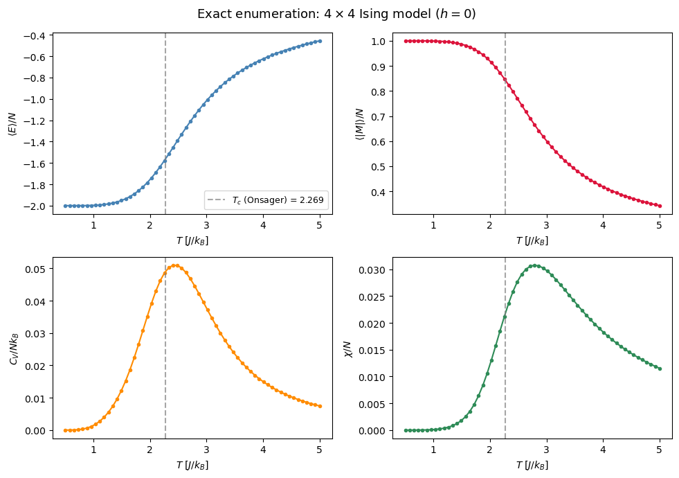
Even on this tiny lattice, the hallmarks of the 2D phase transition are visible: energy drops steeply near , magnetization builds up below , and both and develop peaks near the Onsager critical temperature . On larger lattices — accessible only via Monte Carlo — these peaks sharpen and diverge in the thermodynamic limit.