MD/MC simulations of fluids
Molecular Dynamics Simulation of a Lennard-Jones Fluid
The code in this notebook simulates a collection of particles interacting through the Lennard-Jones (LJ) potential using Molecular Dynamics (MD) in 3D.
The simulation is designed to be efficient, modular, and easy to understand, leveraging NumPy and object-oriented programming (OOP).Particles are initially arranged in a face-centered cubic (FCC) lattice and evolved over time using the Velocity Verlet algorithm under periodic boundary conditions.
The simulation tracks: Kinetic Energy (KE), Potential Energy (PE), Pressure, Pair correlation function
Physical Model of LJ fluid
Each particle experiences a force given by the Lennard-Jones potential:
is the distance between two particles.
The potential is cut off at a radius (r_c) to improve efficiency.
The system is simulated at a fixed temperature by rescaling velocities during the early steps (velocity rescaling).
PBC
If a particle leaves the box, it re-enters at the opposite side.
What should be the distance between partiles? There is some mbiguity because distance between atoms may now include crossing the system boundary and re-entering. This is identical to introducing copies of the particles around the simulation box. We adopt minimum image convention by choosing the shortest distance possible
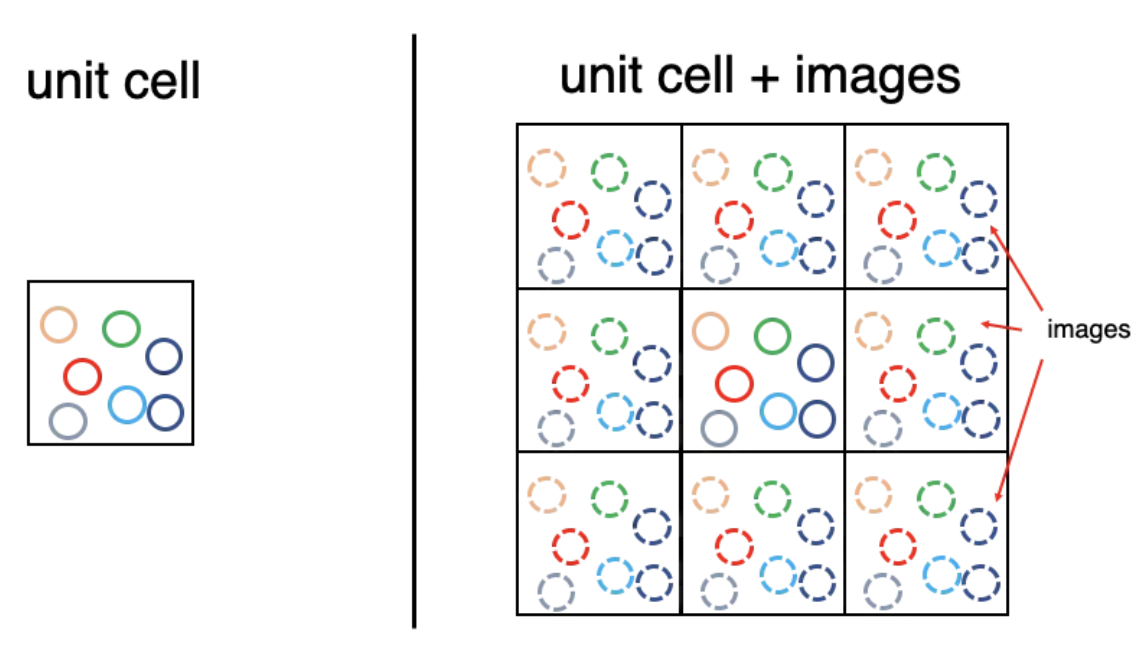
Perioidc Boundary Conditions
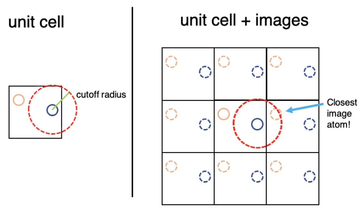
Minimum Image Convention showing that we only track particles with clsoest distance.
MD of LJ fluid
Source
import numpy as np
import matplotlib.pyplot as plt


class LJBase:
    '''Cubic box of N = 4 * N_cell**3 LJ particles on an FCC lattice
    with periodic boundary conditions and minimum-image pair distances.
    Shared geometry/state for the MD and MC subclasses below.'''

    def __init__(self, rho=0.88, N_cell=3, T=1.0, rcut=2.5):
        self.N = 4 * N_cell**3
        self.rho = rho
        self.L = (self.N / rho) ** (1 / 3)
        self.T = T
        self.rcut = rcut
        self.rcut_sq = rcut ** 2

        # FCC lattice: 4-atom basis replicated N_cell**3 times
        base = np.array([[0, 0, 0], [0.5, 0.5, 0], [0.5, 0, 0.5], [0, 0.5, 0.5]])
        pos = np.array([b + [i, j, k]
                        for i in range(N_cell)
                        for j in range(N_cell)
                        for k in range(N_cell)
                        for b in base])
        self.pos = pos * (self.L / N_cell)

        # All N(N-1)/2 unique pair indices, built once
        self.I, self.J = np.triu_indices(self.N, k=1)

    def minimum_image(self, r_vec):
        return (r_vec + self.L / 2) % self.L - self.L / 2


class LJSystem(LJBase):
    '''Lennard-Jones fluid integrated with velocity Verlet (NVE / rescaled NVT).'''

    def __init__(self, rho=0.88, N_cell=3, T=1.0, rcut=2.5):
        super().__init__(rho, N_cell, T, rcut)
        self.T_target = T
        self.vel = np.random.randn(self.N, 3)
        self.vel -= np.mean(self.vel, axis=0)

    def compute_forces(self):
        r_vec = self.minimum_image(self.pos[self.I] - self.pos[self.J])
        r_sq = np.sum(r_vec ** 2, axis=1)

        mask = r_sq < self.rcut_sq
        r_vec = r_vec[mask]
        r_sq = r_sq[mask]

        r2_inv = 1.0 / r_sq
        r6_inv = r2_inv ** 3

        # f_over_r * r_vec = vector force.  f_over_r = -(1/r) dU/dr for LJ:
        #   dU/dr = -24/r * (2/r^12 - 1/r^6)  =>  f_over_r = 48/r^2 (1/r^12 - 1/(2 r^6))
        f_over_r = 48 * r6_inv * (r6_inv - 0.5) * r2_inv
        F_ij = f_over_r[:, None] * r_vec

        forces = np.zeros_like(self.pos)
        np.add.at(forces, self.I[mask],  F_ij)        # scatter pair forces (Newton's 3rd law)
        np.add.at(forces, self.J[mask], -F_ij)

        U = 4 * np.sum(r6_inv * (r6_inv - 1))
        Pvir = np.sum(F_ij * r_vec)                   # virial sum (NOT pressure: see note below)
        hist, _ = np.histogram(np.sqrt(r_sq), bins=30, range=(0, self.L / 2))
        return forces, U, Pvir, hist

    def integrate(self, dt):
        forces, U, Pvir, hist = self.compute_forces()
        self.vel += 0.5 * dt * forces
        self.pos = (self.pos + dt * self.vel) % self.L
        forces_new, U_new, Pvir_new, hist_new = self.compute_forces()
        self.vel += 0.5 * dt * forces_new
        kin = 0.5 * np.sum(self.vel ** 2)
        return kin, U_new, Pvir_new, hist_new

    def rescale_velocities(self, kin):
        '''Berendsen-style velocity rescale to hit the target temperature.'''
        factor = np.sqrt(3 * self.N * self.T_target / (2 * kin))
        self.vel *= factor

    def simulate(self, dt=0.005, nsteps=5000, freq_out=50, n_thermalize=1000):
        kins, pots, Ps, hists = [], [], [], []
        for step in range(nsteps):
            kin, pot, Pvir, hist = self.integrate(dt)
            if step < n_thermalize:
                self.rescale_velocities(kin)
            if step % freq_out == 0:
                kins.append(kin); pots.append(pot)
                Ps.append(Pvir); hists.append(hist)
        return np.array(kins), np.array(pots), np.array(Ps), np.mean(hists, axis=0)
Example simulation and analysis
# Initialize system
lj = LJSystem(rho=0.88, N_cell=3, T=1.0)
# Run simulation
kins, pots, Ps, hist = lj.simulate(dt=0.005, nsteps=10000, freq_out=50)
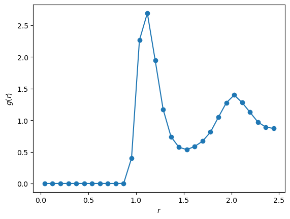
# Post-processing: convert pair-distance histogram to g(r).
# Each unordered pair (i<j) is counted once, so the factor of 2 below is required.
n_bins = len(hist)
edges = np.linspace(0, lj.L/2, n_bins + 1)
r = 0.5 * (edges[:-1] + edges[1:]) # bin centers
dr = edges[1] - edges[0]
shell_volumes = 4*np.pi*r**2*dr # 3D shell volume
g_r = 2.0 * hist / (lj.N * lj.rho * shell_volumes)
# Plot
plt.plot(r, g_r, '-o')
plt.xlabel(r'$r$')
plt.ylabel(r'$g(r)$')
plt.show()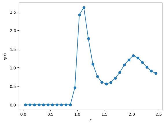
Trajectory diagnostics
The simulate() method already returned kinetic energies (kins), potential energies (pots), and virial sums (Ps) recorded every freq_out steps. Plotting these as time series is the first thing to do for any MD run — it tells you whether the system equilibrated, whether energy is being conserved during the production phase, and whether the temperature is what you asked for.
The instantaneous temperature is read off the kinetic energy via equipartition (in 3D, ):
# Time axis: each saved frame is freq_out integrator steps
freq_out = 50
dt = 0.005
t_ax = np.arange(len(kins)) * freq_out * dt
T_traj = 2.0 * kins / (3.0 * lj.N)
E_total = kins + pots

fig, axes = plt.subplots(2, 2, figsize=(11, 6), sharex=True)
axes[0, 0].plot(t_ax, kins,    color='crimson',   lw=1.2);  axes[0, 0].set_ylabel('Kinetic energy')
axes[0, 1].plot(t_ax, pots,    color='steelblue', lw=1.2);  axes[0, 1].set_ylabel('Potential energy')
axes[1, 0].plot(t_ax, E_total, color='black',     lw=1.2);  axes[1, 0].set_ylabel('Total energy')
axes[1, 1].plot(t_ax, T_traj,  color='goldenrod', lw=1.2)
axes[1, 1].axhline(lj.T_target, color='k', ls='--', lw=0.8, label=f'$T_{{\\rm target}} = {lj.T_target}$')
axes[1, 1].set_ylabel('Temperature')
axes[1, 1].legend()

# Mark end of velocity rescaling (first 1000 steps)
t_thermalize = 1000 * dt
for ax in axes.ravel():
    ax.axvspan(0, t_thermalize, color='gray', alpha=0.15)
    ax.grid(True, ls=':', alpha=0.5)
for ax in axes[1]:
    ax.set_xlabel('time (LJ units)')
fig.suptitle('Thermalization (gray band) followed by NVE production', y=1.02)
fig.tight_layout()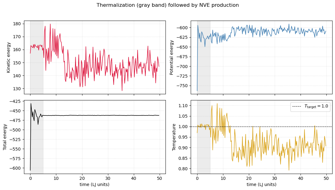
The total energy is essentially constant after the rescaling band ends — that is the signature of a properly working symplectic integrator. The temperature fluctuates around its target with relative magnitude , exactly as predicted for the canonical ensemble in the thermodynamic limit.
Watching the fluid in 3D
A short, instrumented re-run lets us snapshot positions during the simulation and animate them. Each frame below is the full box at one instant — particles disappearing on one face and reappearing on the opposite face is just periodic boundary conditions.
from matplotlib.animation import FuncAnimation
from IPython.display import HTML

# Fresh system; record snapshots while it runs
lj_anim = LJSystem(rho=0.7, N_cell=3, T=1.0)
n_steps_anim = 1500
save_every = 30
n_thermalize = 400

snapshots = [lj_anim.pos.copy()]
unwrapped = lj_anim.pos.copy()
prev_wrapped = lj_anim.pos.copy()
unwrapped_traj = [unwrapped.copy()]

for step in range(n_steps_anim):
    kin, _, _, _ = lj_anim.integrate(0.005)
    if step < n_thermalize:
        lj_anim.rescale_velocities(kin)
    # Track unwrapped positions for the MSD analysis below
    delta = lj_anim.pos - prev_wrapped
    delta -= lj_anim.L * np.round(delta / lj_anim.L)
    unwrapped = unwrapped + delta
    prev_wrapped = lj_anim.pos.copy()
    if step % save_every == 0 and step >= n_thermalize:
        snapshots.append(lj_anim.pos.copy())
        unwrapped_traj.append(unwrapped.copy())

snapshots = np.array(snapshots)
unwrapped_traj = np.array(unwrapped_traj)

fig = plt.figure(figsize=(5, 5))
ax = fig.add_subplot(111, projection='3d')
sc = ax.scatter(snapshots[0, :, 0], snapshots[0, :, 1], snapshots[0, :, 2],
                s=80, c='steelblue', edgecolors='k', alpha=0.85)
ax.set_xlim(0, lj_anim.L); ax.set_ylim(0, lj_anim.L); ax.set_zlim(0, lj_anim.L)
ax.set_xticks([]); ax.set_yticks([]); ax.set_zticks([])
title = ax.set_title(f'frame 0 / {len(snapshots)-1}')

def update(k):
    sc._offsets3d = (snapshots[k, :, 0], snapshots[k, :, 1], snapshots[k, :, 2])
    title.set_text(f'frame {k} / {len(snapshots)-1}')
    return sc, title

ani = FuncAnimation(fig, update, frames=len(snapshots), interval=120, blit=False)
plt.close()
HTML(ani.to_jshtml())Diffusion from the mean squared displacement
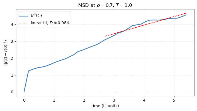
In a liquid, particles wander around. The mean squared displacement of unwrapped trajectories grows linearly with time at long times,
with the self-diffusion coefficient. This is one of the most important observables MD gives you — and one MC cannot, because MC has no real time. A linear fit to the long- portion of the MSD (avoiding the early ballistic regime where ) recovers .
# MSD averaged over particles, with respect to the first saved frame
disp = unwrapped_traj - unwrapped_traj[0]
msd = np.mean(np.sum(disp ** 2, axis=-1), axis=-1)
t_msd = np.arange(len(msd)) * save_every * 0.005

# Linear fit on the second half (avoid ballistic short-time regime)
from scipy.stats import linregress
mid = len(msd) // 2
slope, intercept, *_ = linregress(t_msd[mid:], msd[mid:])
D = slope / 6.0    # 3D Einstein relation

fig, ax = plt.subplots(figsize=(7, 4))
ax.plot(t_msd, msd, color='steelblue', lw=2, label='$\\langle r^2(t)\\rangle$')
ax.plot(t_msd[mid:], slope * t_msd[mid:] + intercept, 'r--', lw=1.5,
        label=fr'linear fit, $D \approx {D:.3f}$')
ax.set(xlabel='time (LJ units)', ylabel=r'$\langle |r(t) - r(0)|^2\rangle$',
       title=fr'MSD at $\rho={lj_anim.rho}$, $T={lj_anim.T_target}$')
ax.legend()
ax.grid(True, ls=':', alpha=0.5)
fig.tight_layout()
print(f'Self-diffusion coefficient D ≈ {D:.4f} (LJ units)')
Self-diffusion coefficient D ≈ 0.0844 (LJ units)
MC simulation
Recall the Metropolis criterion from the MCMC labs and from the 2D LJ MC in Intro2Fluids: pick a particle, propose a small displacement, accept with probability
We apply it below to the same 3D LJ fluid as our MD run above so we can compare the two methods directly.
Source
class LJ_MC_System(LJBase):
    '''Lennard-Jones fluid sampled with Metropolis Monte Carlo.'''

    def __init__(self, rho=0.88, N_cell=3, T=1.0, rcut=2.5):
        super().__init__(rho, N_cell, T, rcut)
        self.beta = 1.0 / T

    def total_energy(self):
        r_vec = self.minimum_image(self.pos[self.I] - self.pos[self.J])
        r_sq = np.sum(r_vec ** 2, axis=1)
        mask = r_sq < self.rcut_sq
        r6_inv = (1.0 / r_sq[mask]) ** 3
        return 4 * np.sum(r6_inv * (r6_inv - 1))

    def particle_energy(self, idx):
        rij = self.minimum_image(self.pos[idx] - self.pos)
        r_sq = np.sum(rij ** 2, axis=1)
        mask = (r_sq < self.rcut_sq) & (r_sq > 0)     # exclude self
        r6_inv = (1.0 / r_sq[mask]) ** 3
        return 4 * np.sum(r6_inv * (r6_inv - 1))

    def mc_move(self, max_disp=0.1):
        idx = np.random.randint(self.N)
        old_pos = self.pos[idx].copy()
        old_e = self.particle_energy(idx)

        self.pos[idx] = (self.pos[idx] + (np.random.rand(3) - 0.5) * 2 * max_disp) % self.L
        new_e = self.particle_energy(idx)

        if np.random.rand() > np.exp(-self.beta * (new_e - old_e)):
            self.pos[idx] = old_pos                   # reject

    def sample(self):
        '''One pair-distance histogram for g(r).'''
        r_vec = self.minimum_image(self.pos[self.I] - self.pos[self.J])
        r_sq = np.sum(r_vec ** 2, axis=1)
        hist, _ = np.histogram(np.sqrt(r_sq), bins=30, range=(0, self.L / 2))
        return hist

    def simulate(self, nsteps=50000, freq_out=500, max_disp=0.1):
        hists, energies = [], []
        for step in range(nsteps):
            self.mc_move(max_disp=max_disp)
            if step % freq_out == 0:
                hists.append(self.sample())
                energies.append(self.total_energy())
        return np.array(energies), np.mean(hists, axis=0)
Example MC simulation and analysis
# ----------------- Main -----------------

# Initialize system
lj_mc = LJ_MC_System(rho=0.88, N_cell=3, T=1.0)

# Run simulation
energies, hist = lj_mc.simulate(nsteps=100000, freq_out=500)

# Post-processing: convert pair-distance histogram to g(r).
n_bins = len(hist)
edges = np.linspace(0, lj_mc.L/2, n_bins + 1)
r = 0.5 * (edges[:-1] + edges[1:])              # bin centers
dr = edges[1] - edges[0]
shell_volumes = 4*np.pi*r**2*dr
g_r = 2.0 * hist / (lj_mc.N * lj_mc.rho * shell_volumes)

# Plot
plt.plot(r, g_r, '-o')
plt.xlabel(r'$r$')
plt.ylabel(r'$g(r)$')
plt.show()
Tagged particle: MD trajectory vs. MC walk
Both methods sample the same equilibrium distribution, so comes out the same. But the time series of any single particle looks completely different. In MD each step is a finite slice of real physical time and the trajectory is dynamical — particles ballistically translate, collide, and diffuse. In MC each step is a random local proposal accepted with the Metropolis rule, so the trajectory is a random walk with no inertia and no real time.
Tracking the unwrapped -coordinate of particle 0 in both runs makes the contrast visible.
# MC: do many sweeps (one sweep = N attempted moves) and record particle 0
def mc_sweep(lj_mc, max_disp=0.1):
    for _ in range(lj_mc.N):
        lj_mc.mc_move(max_disp=max_disp)

lj_mc_track = LJ_MC_System(rho=0.7, N_cell=3, T=1.0)
n_sweeps_mc = 200
mc_unwrapped = lj_mc_track.pos[0, 0]
prev_x = lj_mc_track.pos[0, 0]
mc_traj_x = [mc_unwrapped]
for s in range(n_sweeps_mc):
    mc_sweep(lj_mc_track, max_disp=0.15)
    cur_x = lj_mc_track.pos[0, 0]
    delta = cur_x - prev_x
    delta -= lj_mc_track.L * round(delta / lj_mc_track.L)   # unwrap PBC
    mc_unwrapped += delta
    prev_x = cur_x
    mc_traj_x.append(mc_unwrapped)
mc_traj_x = np.array(mc_traj_x)

# MD trace: re-use unwrapped_traj from the animation cell above
md_traj_x = unwrapped_traj[:, 0, 0]
t_md_axis = np.arange(len(md_traj_x)) * save_every * 0.005

fig, axes = plt.subplots(1, 2, figsize=(12, 4), sharey=True)
axes[0].plot(t_md_axis, md_traj_x, color='steelblue', lw=1.2)
axes[0].set(xlabel='time (LJ units)', ylabel='$x$ of tagged particle (unwrapped)',
            title='MD: smooth dynamical trajectory')
axes[0].grid(True, ls=':', alpha=0.5)

axes[1].plot(np.arange(len(mc_traj_x)), mc_traj_x, color='crimson', lw=1.2)
axes[1].set(xlabel='MC sweep', title='MC: random walk, no real time')
axes[1].grid(True, ls=':', alpha=0.5)
fig.tight_layout()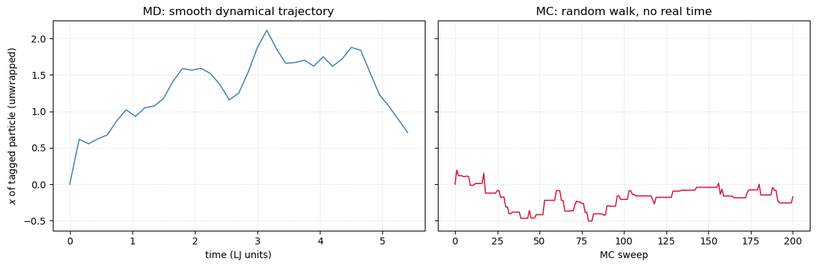
Differences of Monte Carlo vs Molecular Dynamics
| Monte Carlo (MC) | Molecular Dynamics (MD) |
|---|---|
| No real dynamics, just configurations | Real-time evolution of particle trajectories |
| Samples equilibrium ensemble directly | Samples via time evolution |
| No conservation laws | Energy/momentum conserved after equilibration |
| Easier to implement | More complex (forces, integration needed) |
| Faster for static properties like | Necessary for dynamics (diffusion, viscosity) |
Beyond hand-coded forces
The LJ force routine above had to be derived analytically from the potential. An alternative is to write only the energy and let automatic differentiation produce forces, pressures, and parameter sensitivities for free — the basis of modern differentiable simulation. For a self-contained walk-through using JAX, see labs
Problems
MD sim of LJ fluid
Modify the cut-off radius and observe its effect on pressure and energy.
Remove velocity rescaling after equilibration and check energy conservation.
Implement a thermostat (e.g., Andersen, Berendsen) instead of manual rescaling.
Compute the diffusion coefficient from particle trajectories.
Visualize the particle trajectories over time (animation!).
MC sim of LJ fluid
Vary sim parameters
Tune maximum displacement (
max_disp) to optimize acceptance rate (~40%-50% is ideal).Check how changes when density or temperature changes.
Implement energy cutoffs with shifted potentials to smooth out the energy at .
Try simulating hard spheres (infinite repulsion at contact).
Phases of LJ fluid
Run MD or MC simulations of LJ fluid at several temperatures to identify critical temperature.
At each temperature evaluate heat capacity and RDFs.
Plot how energy, heat capacity and RDF change as a function of temperature.
Study dependence on sampling efficiency on magnitude of particle displacement.
Reference
D. Frenkel and B. Smit, Understanding Molecular Simulation: From Algorithms to Applications, 2nd ed. (Academic Press, 2002) — chapter 4 on molecular dynamics, chapter 3 on Monte-Carlo, and Appendix F on the Lennard-Jones equation of state.
J. K. Johnson, J. A. Zollweg, K. E. Gubbins, The Lennard-Jones equation of state revisited, Mol. Phys. 78, 591 (1993). Johnson et al. (1993)
- Johnson, J. K., Zollweg, J. A., & Gubbins, K. E. (1993). The Lennard-Jones equation of state revisited. Molecular Physics, 78(3), 591–618. 10.1080/00268979300100411