Intro to Statistical Ensembles

What you will learn

Statistical Ensembles: Understanding the role of ensembles in statistical mechanics and how they describe macroscopic systems using probability distributions.
Microcanonical Ensemble (NVE): Definition, characteristics, and assumptions—fixed energy, volume, and particle number; statistical weight of microstates.
Canonical Ensemble (NVT): Definition and significance—fixed temperature, volume, and particle number; derivation of the Boltzmann factor.
Equivalence of Ensembles: Conditions under which the microcanonical and canonical ensembles give equivalent thermodynamic predictions in the thermodynamic limit.
Partition Function ( $Z$ ): Role of the partition function in statistical mechanics, its connection to thermodynamic properties (free energy, entropy, internal energy).
Boltzmann Distribution: Probability of a system being in a given energy state at equilibrium, leading to macroscopic observables.
Thermodynamic Connections: How ensemble averages link to macroscopic properties such as energy, entropy, and pressure.
Fluctuations and Large System Limits: How energy fluctuations in the canonical ensemble become negligible for large systems, reinforcing ensemble equivalence.

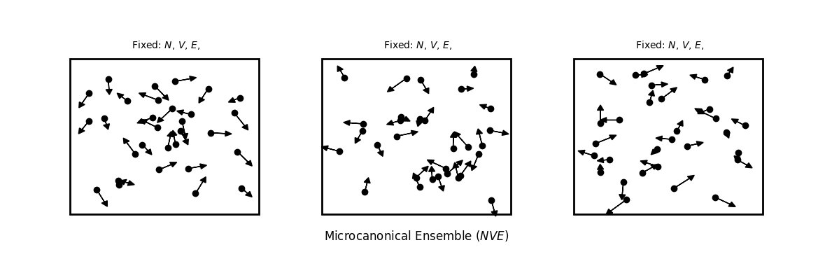
Microcanonical Ensemble (NVE)¶

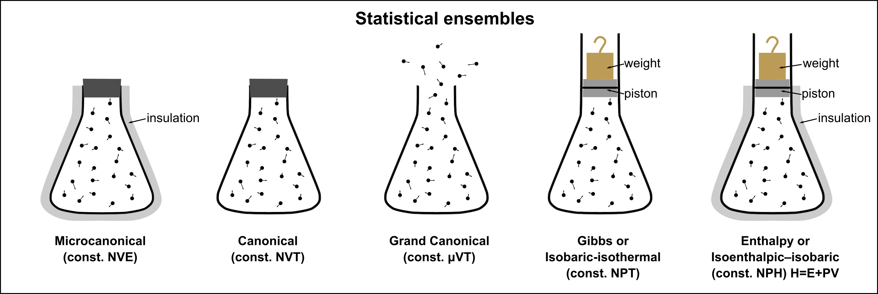
A collection of all possible microscopic arrangements consistend with an equilibrium thermodynamic state is called statistical ensemble.
Ensemble defines sample space over microstates over which we define micro and macro-state probabilities
Consider an isolated fluid system with $N=const$ , $V=const$ and $E=const$ . This is called a microcanonical ensemble
In the absence of any physical constraints, no micro state is more probable than any other. This is known as “principle of equal a priory probability”.

import matplotlib.pyplot as plt
import numpy as np

# Function to draw an isolated system (box with particles and motion arrows)
def draw_system(ax, x_offset=0):
    # Draw the box
    box = plt.Rectangle((x_offset, 0), 3, 3, edgecolor='black', linewidth=2, facecolor='none')
    ax.add_patch(box)
    
    # Fixed parameters label
    ax.text(x_offset + 1.5, 3.2, r' Fixed: $ N$, $V$, $ E$,', ha='center', fontsize=10)
    
    # Randomly place particles
    np.random.seed(x_offset)  # Ensure different particles per box
    num_particles = 30
    particle_positions = np.random.rand(num_particles, 2) * 2.5 + np.array([x_offset + 0.25, 0.25])

    for px, py in particle_positions:
        ax.plot(px, py, 'ko', markersize=6)  # Particles as black dots
        # Add motion arrows
        dx, dy = np.random.uniform(-0.5, 0.5), np.random.uniform(-0.5, 0.5)
        ax.arrow(px, py, dx * 0.5, dy * 0.5, head_width=0.1, head_length=0.1, fc='black', ec='black')

# Create figure
fig, ax = plt.subplots(figsize=(12, 4))
ax.set_xlim(-1, 12)
ax.set_ylim(-1, 4)
ax.set_xticks([])
ax.set_yticks([])
ax.axis('off')

# Draw three isolated systems (microcanonical ensemble representation)
draw_system(ax, x_offset=0)
draw_system(ax, x_offset=4)
draw_system(ax, x_offset=8)

# Label the entire system
ax.text(5.5, -0.5, r'Microcanonical Ensemble ($NVE$)', ha='center', fontsize=12)

# Show plot
plt.tight_layout()

We can use postulate of equal mircro-state probabilities and plug into probabilisti expression of entropy to obtain a simple relationship between number of microstates and entropy:

S = -k_B \sum_i p_i log p_i = -k_B \Omega \cdot \frac{1}{\Omega} log \frac{1}{\Omega}

(2)

Simple example of NVE ensemble

Consider a system of three spins where $\uparrow$ and $\downarrow$ have the same energy $\epsilon$ . We have microcanonical ensemble defined by $N=3$ and $E=3\epsilon$ thermodynamic variables.

\boxed{ \uparrow \uparrow \uparrow, \quad \uparrow \uparrow \downarrow, \quad \uparrow \downarrow \uparrow, \quad \downarrow \uparrow \uparrow, \quad \uparrow \downarrow \downarrow, \quad \downarrow \uparrow \downarrow, \quad \downarrow \downarrow \uparrow, \quad \downarrow \downarrow \downarrow}

(4)

There are $\Omega = 2^3$ microstates with entropy being:

S = k_B \log 2^3 = 3k_B log2

(5)

For N spins we see that $\Omega=2^N$ and therefore entropy scales linearly with system size $N$

S = Nk_B log2

(6)

Microcanonical partition function grows exponentially with system size¶

# Increase the number of particles
num_particles = 200  # More particles
Lx, Ly=10,10
cell_size=2.5
# Generate new random particle positions
x_positions = np.random.uniform(0, Lx, num_particles)
y_positions = np.random.uniform(0, Ly, num_particles)

# Create plot
plt.figure(figsize=(4, 4))

# Plot particles
plt.scatter(x_positions, y_positions, color='blue', s=20, alpha=0.7)

# Draw grid
for x in np.arange(0, Lx + cell_size, cell_size):
    plt.axvline(x, color='black', linestyle='-', linewidth=0.8)
for y in np.arange(0, Ly + cell_size, cell_size):
    plt.axhline(y, color='black', linestyle='-', linewidth=0.8)

# Labels and title
plt.xlabel("x")
plt.ylabel("y")
plt.title("Particles in a 2D Box with Statistically Independent Grid Cells")
plt.xlim(0, Lx)
plt.ylim(0, Ly)
plt.grid(False)  # Disable matplotlib default grid to use custom grid

plt.show()

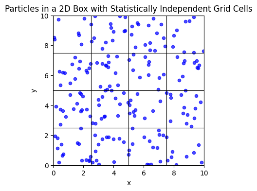
To estimate how the number of microstates behave as a function of system size consider $N$ particles in a volume $V$ , and particle density $\rho = \frac{N}{V}$
Dividing the system into $M$ statistically independent subregions of volume $M = V/v$ containing $\Omega_{\text{sub}}$ microstates in each we get:

\Omega(E) = \left( \Omega_{\text{sub}} \right)^M = \left( \Omega^{1/\rho v}_{\text{sub}} \right)^N

(7)

We find that number of mirostates grows exponentially with syste size $N$ . This implies a large deviation property: entropy scales extensively and grows monotonically with energy.

Applications of NVE¶

Particles in a box¶

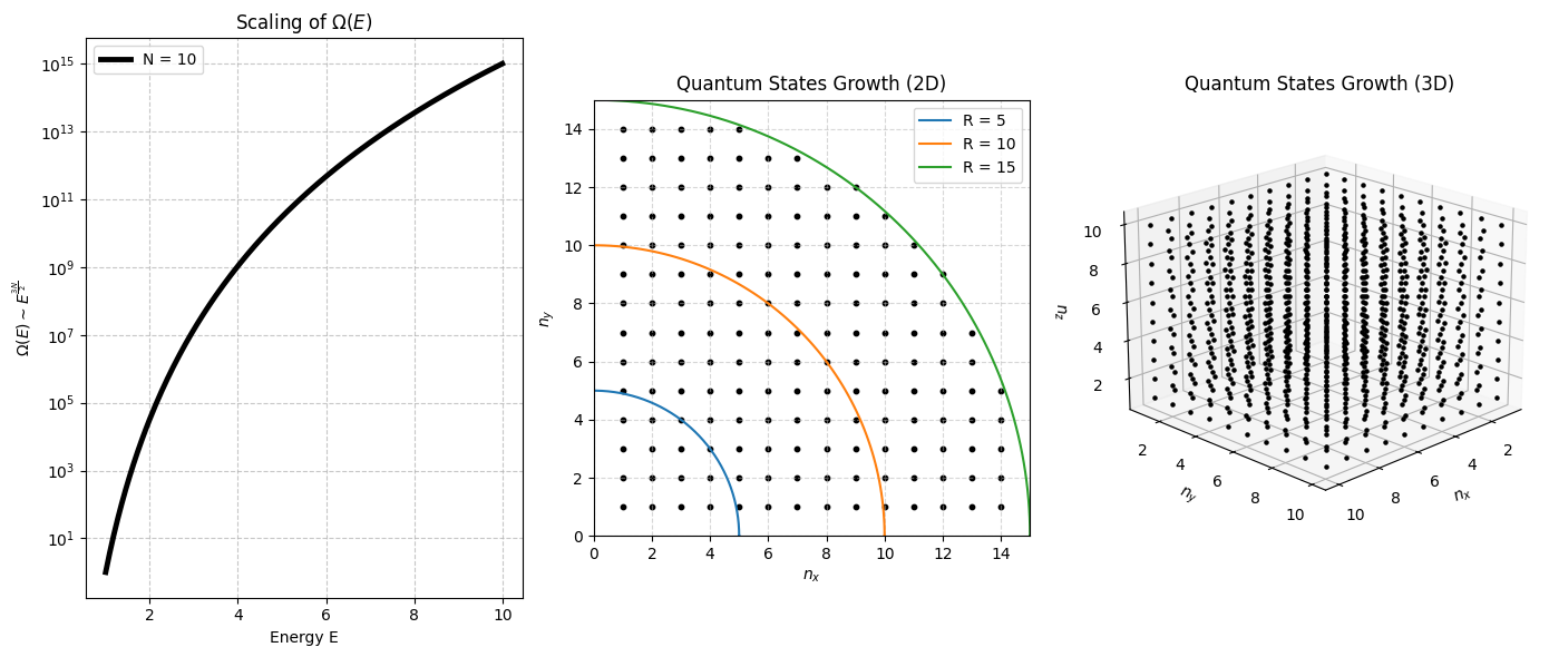
For a single quantum particle in a cubical box of side $L$ , the allowed energy levels are:

E_{n_x, n_y, n_z} \sim (n_x^2 + n_y^2 + n_z^2)

(10)

Where $n_x, n_y, n_z$ are positive integers (quantum numbers).
To determine the number of microstates with total energy at most $E$ , we count the number of allowed quantum states $(n_x, n_y, n_z)$ satisfying:

n_x^2 + n_y^2 + n_z^2 \leq E

(11)

For large $E$ , this corresponds to counting integer lattice points inside a sphere of radius:

R = \sqrt{E}

(12)

Since the number of points inside a sphere scales approximately as the volume of the sphere, we get:

\Omega(E) \approx \frac{4}{3} \pi R^3 \propto E^{3/2}

(13)

Thus, for a single particle, the number of accessible microstates grows as:

\Omega(E) \sim E^{3/2}

(14)

For $N$ independent particles, each particle contributes an independent set of quantum numbers, meaning we now count lattice points in a $3N$ -dimensional hypersphere.

\Omega(E) \sim E^{3N/2}

(15)

# Create a combined figure
fig = plt.figure(figsize=(14, 6))

# ---------------- Plot 1: Scaling of Microstates ----------------
ax1 = fig.add_subplot(131)
E = np.linspace(1, 10, 200)

N=10

Omega = E**(1.5 * N)
ax1.plot(E, Omega, label=f"N = {N}", color='black', lw=3.5)

ax1.set_xlabel("Energy E")
ax1.set_ylabel(r"$\Omega(E) \sim E^{\frac{3N}{2}}$")
ax1.set_title("Scaling of $\Omega(E)$")
ax1.set_yscale('log')  # Logarithmic scale to better display the exponential growth
ax1.grid(True, linestyle='--', alpha=0.7)
ax1.legend()

# ---------------- Plot 2: Growth of Quantum States in 2D ----------------
ax2 = fig.add_subplot(132)
n_max = 15  # Reduce max quantum number for clarity
R_values = [5, 10, 15]
n_x_values = np.arange(1, n_max + 1)
n_y_values = np.arange(1, n_max + 1)

for n_x in n_x_values:
    for n_y in n_y_values:
        energy = n_x**2 + n_y**2
        if energy <= max(R_values)**2:
            ax2.scatter(n_x, n_y, color='black', s=10)

theta = np.linspace(0, 2 * np.pi, 300)
for R in R_values:
    ax2.plot(R * np.cos(theta), R * np.sin(theta), label=f'R = {R}', linewidth=1.5)

ax2.set_xlabel(r'$n_x$')
ax2.set_ylabel(r'$n_y$')
ax2.set_title('Quantum States Growth (2D)')
ax2.legend()
ax2.set_xlim(0, n_max)
ax2.set_ylim(0, n_max)
ax2.grid(True, linestyle='--', alpha=0.5)
ax2.set_aspect('equal')

# ---------------- Plot 3: 3D Representation of Quantum States ----------------
ax3 = fig.add_subplot(133, projection='3d')
n_max_3d = 10  # Reduce quantum number range for clarity

# Generate 3D quantum states
n_z_values = np.arange(1, n_max_3d + 1)
for n_x in np.arange(1, n_max_3d + 1):
    for n_y in np.arange(1, n_max_3d + 1):
        for n_z in np.arange(1, n_max_3d + 1):
            energy = n_x**2 + n_y**2 + n_z**2
            if energy <= max(R_values)**2:
                ax3.scatter(n_x, n_y, n_z, color='black', s=5)

ax3.set_xlabel(r'$n_x$')
ax3.set_ylabel(r'$n_y$')
ax3.set_zlabel(r'$n_z$')
ax3.set_title('Quantum States Growth (3D)')
ax3.view_init(elev=20, azim=45)

# Show the combined figure
plt.tight_layout()
plt.show()

<>:15: SyntaxWarning: invalid escape sequence '\O'
<>:15: SyntaxWarning: invalid escape sequence '\O'
/tmp/ipykernel_2848/3458926410.py:15: SyntaxWarning: invalid escape sequence '\O'
  ax1.set_title("Scaling of $\Omega(E)$")

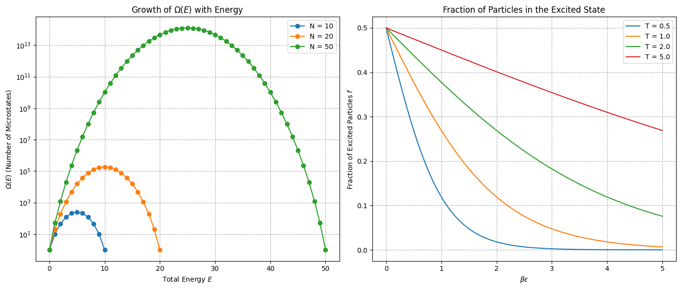
Two state system¶

Given $N$ non-interacting spins where each spin can be up ( $\uparrow$ ) with energy $\epsilon$ or down ( $\downarrow$ ) with energy $0$ . The total energy is:
$E = n\epsilon$
(16)
Determine fraction of excited states $f=\frac{n}{N} = \frac{E}{N\epsilon}$ where $n$ is number of up spins. Show how this fraciton changes with temperature

log\Omega(E, N) = log \frac{N!}{n! (N-n)!} = \frac{N!}{(E/\epsilon)! (N-E/\epsilon)!}

(17)

Using Striling’s approximation $logN!=NlogN-N$ we get:

log\Omega(E, N) \approx N \log N - \frac{E}{\epsilon} \log \frac{E}{\epsilon} - \bigg(N - \frac{E}{\epsilon}\bigg) \log \bigg(N - \frac{E}{\epsilon}\bigg)

(18)

We connect number of excited states to equilibrium temperature via thermodynamics

\frac{1}{T} = \frac{dS}{dE} = k_B \frac{d log\Omega}{dE}

(19)

\frac{1}{k_BT} = - \frac{1}{\epsilon} \log \frac{E}{\epsilon} + \frac{1}{\epsilon} \log \bigg(N - \frac{E}{\epsilon}\bigg)

(20)

\frac{E}{\epsilon} = \bigg(N - \frac{E}{\epsilon}\bigg) e^{-\frac{\epsilon}{k_B T} }

(21)

f = \frac{E}{N\epsilon} = \frac{1}{1 + e^{\frac{\epsilon}{k_B T} }}

(22)

This is the well-known Boltzmann factor result for a two-level system in thermal equilibrium. At high temperatures ( $k_B T \gg \epsilon$ ), approximately half the particles are excited, while at low temperatures ( $k_B T \ll \epsilon$ ).

import numpy as np
import scipy.special as sp
import matplotlib.pyplot as plt

# Create a figure with two subplots
fig, axes = plt.subplots(1, 2, figsize=(14, 6))

# Subplot 1: Growth of Ω(E) with Energy for Different Spin System Sizes
N_values = [10, 20, 50]  # Different spin system sizes

for N in N_values:
    energies = np.arange(0, N+1, 1)  # Possible energy levels
    multiplicities = sp.binom(N, energies)  # Compute binomial coefficient
    axes[0].plot(energies, multiplicities, label=f'N = {N}', linestyle='-', marker='o')

# Plot settings for first subplot
axes[0].set_yscale('log')  # Use logarithmic scale to highlight exponential growth
axes[0].set_xlabel(r'Total Energy $E$')
axes[0].set_ylabel(r'$\Omega(E)$ (Number of Microstates)')
axes[0].set_title(r'Growth of $\Omega(E)$ with Energy')
axes[0].legend()
axes[0].grid(True, which='both', linestyle='--')

# Subplot 2: Fraction of Particles in the Excited State vs. Temperature
epsilon = 1.0  # Set energy scale to 1 for simplicity
k_B = 1.0  # Boltzmann constant set to 1 for simplicity
T_values = [0.5, 1.0, 2.0, 5.0]  # Different temperature values

# Define function for fraction of excited particles
def fraction_excited(beta_epsilon):
    return 1 / (1 + np.exp(beta_epsilon))

# Generate beta_epsilon values
beta_epsilon_values = np.linspace(0, 5, 100)

# Plot f for different temperatures
for T in T_values:
    beta_epsilon = epsilon / (k_B * T) * beta_epsilon_values
    f_values = fraction_excited(beta_epsilon)
    axes[1].plot(beta_epsilon_values, f_values, label=f"T = {T}")

# Plot settings for second subplot
axes[1].set_xlabel(r"$\beta \epsilon$")
axes[1].set_ylabel(r"Fraction of Excited Particles $f$")
axes[1].set_title("Fraction of Particles in the Excited State")
axes[1].legend()
axes[1].grid(True, linestyle='--')

# Adjust layout
plt.tight_layout()
plt.show()

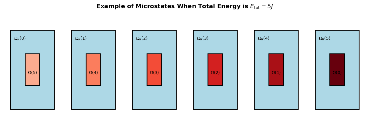
Energy partitioning in an isolated system¶

import matplotlib.pyplot as plt

# Create figure
fig, ax = plt.subplots(figsize=(7, 6))
ax.set_xlim(-1, 7)
ax.set_ylim(-1, 5)
ax.set_xticks([])
ax.set_yticks([])
ax.axis('off')

# Draw the large reservoir (outer rectangle)
reservoir = plt.Rectangle((0, 0), 6, 4, edgecolor='black', facecolor='lightblue', linewidth=2, label="Reservoir (Ω_R)")
ax.add_patch(reservoir)

# Draw the small system (inner rectangle)
small_system = plt.Rectangle((2, 1.2), 2, 1.6, edgecolor='black', facecolor='lightcoral', linewidth=2, label="Small System (Ω_S)")
ax.add_patch(small_system)

# Annotate the system and reservoir
#ax.text(3, -0.5, r'\textbf{System with Reservoir: Energy Exchange}', ha='center', fontsize=12)
ax.text(0.3, 3.5, r'Reservoir $\Omega_R(E_T-E)$', fontsize=12, color='black', fontweight='bold')
ax.text(2.5, 1.8, r'System $\Omega(E)$', fontsize=12, color='black', fontweight='bold')

# Draw arrows indicating energy exchange
ax.arrow(4, 2, 1, 0, head_width=0.2, head_length=0.2, fc='black', ec='black')
ax.arrow(5, 2, -1, 0, head_width=0.2, head_length=0.2, fc='black', ec='black')

# Label energy exchange
ax.text(5, 2.3, r'$E$', fontsize=12, color='black', fontweight='bold')

# Show plot
# Add a centered title
plt.suptitle(r'Microcanonical Ensemble of system + reservoir with $E_{tot}$ total energy partitioned between them', fontsize=14, fontweight='bold', y=1.05)

plt.tight_layout()

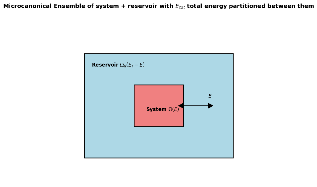
$\Omega_T(E_t)$ is the total number of microstates of the whole isoluate box divided into:
- $\Omega(E)$ number of microstates available to the system of interest
- $\Omega_R(E_T - E)$ number of microstates available to the Reservoir
Since reservoir and system can be considered statistically independent, the probability of finding the system in a macrostate with energy $E$ is:
$p(E) = \frac{\Omega(E) \Omega_R(E_t - E)}{\Omega_T(E_T)}$
(23)
This is a ratio of all microstate where system gets $E$ and reservoir $E_t-E$ energies divided by total number of microstates. The latter given as sum of all possible partitionings of energy
$\Omega_t(E_t) = \sum_E \Omega(E) \Omega_R(E_T - E)$
(24)
We can see that probability of macrostates is normalized $\sum_E P(E)=1$ . The system is more likely to be in a macrostate $E$ if there are more microstates that reaalize this partitioning.

import numpy as np
import matplotlib.pyplot as plt
import matplotlib.cm as cm

# Define total energy levels and number of states
total_energy = 5  # Maximum energy that can be distributed
num_states = total_energy + 1  # Number of possible distributions

# Create figure
fig, axes = plt.subplots(1, num_states, figsize=(12, 4), constrained_layout=True)

# Generate colors based on energy (darker means more energy in the system)
colors = cm.Reds(np.linspace(0.3, 1, num_states))

for i, E_sys in enumerate(range(total_energy, -1, -1)):  # Loop over energy distributions
    E_res = total_energy - E_sys  # Reservoir gets the rest of the energy

    ax = axes[i]
    ax.set_xlim(-1, 7)
    ax.set_ylim(-1, 5)
    ax.set_xticks([])
    ax.set_yticks([])
    ax.axis('off')

    # Draw the reservoir (outer rectangle)
    ax.add_patch(plt.Rectangle((0, 0), 6, 4, edgecolor='black', facecolor='lightblue', linewidth=2))

    # Draw the small system (inner rectangle) with color depending on energy
    ax.add_patch(plt.Rectangle((2, 1.2), 2, 1.6, edgecolor='black', facecolor=colors[i], linewidth=2))

    # Annotate the system and reservoir with energy values
    ax.text(0.5, 3.5, rf'$\Omega_R({E_res})$', fontsize=10, color='black', fontweight='bold')
    ax.text(2.4, 1.8, rf'$\Omega({E_sys})$', fontsize=10, color='black', fontweight='bold')

# Add a centered title
fig.suptitle(r'Example of Microstates When Total Energy is $E_{\mathrm{tot}} = 5 J$', fontsize=14, fontweight='bold', y=1.05)

# Show the ensemble visualization
plt.show()

# Re-import necessary libraries since execution state was reset
import numpy as np
import matplotlib.pyplot as plt

# Define different system sizes
system_sizes = [(5, 10), (10, 20), (20, 40)]

# Define total energy
E_total = 5

# Create figure
plt.figure(figsize=(7, 6))

# Loop over different system sizes and plot
for N1, N2 in system_sizes:
    # Define energy range for system 1 (from 0 to E_total)
    E1_values = np.linspace(0.01, E_total, 50)  # Avoid E=0 to prevent singularities
    E2_values = E_total - E1_values  # Energy remaining for system 2

    # Compute microstates using Omega(E) ~ E^(3N/2)
    Omega1 = E1_values**(3 * N1 / 2)
    Omega2 = E2_values**(3 * N2 / 2)

    # Compute total number of microstates (product of subsystems)
    Omega_total = Omega1 * Omega2 / np.sum(Omega1 * Omega2)  # Normalize to get probability

    # Plot results
    plt.plot(E1_values, Omega_total, label=rf'$N_1={N1}, N_2={N2}$')

    # Draw vertical line at the peak (mean energy E = U)
    E_peak = E1_values[np.argmax(Omega_total)]
    plt.axvline(E_peak, color='black', linestyle=':', linewidth=2)

# Plot settings
plt.xlabel(r"Energy given to System: $E_1$")
plt.ylabel(r"$P(E_1)$")
plt.title("Probability Distribution of Energy Partitioning")
plt.legend()
plt.grid(True)

# Show plot
plt.show()

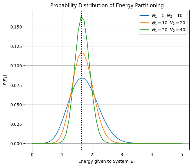
Temperature is the driver of energy partitioning¶

Which paritioning is most likely? For two systems exchanging energy we can write down probability of macrostate and find its maxima with respect to $E$

\frac{d }{dE}logP(E) = \frac{d }{dE} \bigg[ log\Omega(E)\Omega_2(E_{T}-E) \bigg]= 0

(25)

\frac{d}{dE}logP(E) = \bigg[ \frac{d }{dE} log\Omega_1 - \frac{d}{dE}log\Omega_2 \bigg]= 0

(26)

Since $logP(E)\sim S(E)+S_R(E_T-E)$ we note that Maximizing probability of a macrostate is the same as maximizing entropy of macrostate!
We also come to appreacite that inverse temperature $\beta=\frac{1}{k_BT}$ , quantifies rate of growth of microstates.
At lower temperatures $\beta$ is larger indicating faster growth of microstates. At higher temperatures $\beta$ is smaller indicating slower groth of microstates with addition of energy.

Thermal Equilibrium in Ideal Gases¶

For a system of non-interacting particles in a box, the number of microstates follows $\Omega \sim E^{\frac{3}{2}N}$ . The entropy is defined as:
$S_{\text{total}} \sim k_B \log \Omega_1(E_1)\Omega_2(E_{tot}-E_1) = \frac{3}{2} Nk_BlogE_1 + \frac{3}{2} Nk_Blog(E-E_1)$
(28)
Maximizing entropy with respect to energy exchange between two subsystems $E_1$ gives use the equilibrium value $U_1$ that system gets.
$\frac{\partial S_{\text{total}}}{\partial E_1}\bigg|_{E_1=U_1} = \frac{3}{2} k_B \frac{N_1}{U_1} - \frac{3}{2} k_B \frac{N_2}{E-U_1} = 0.$
(29)
Plugging the definition of temperature on left hand side which in equilibrium we see is equal for two systems exchangeing energy:
$\frac{1}{k_B T} = \frac{3}{2} \frac{N_1}{U_1} = \frac{3}{2} \frac{N_2}{U_2}.$
(30)
This leads to the well-known result that each degree of freedom receives $\frac{1}{2} k_B T$ of thermal energy:
$U = \frac{3}{2} N k_B T.$
(31)
Solving for $U_1$ we also see that each system gets energy proportionate to its size
$U_1 = \frac{N_1}{N_1 + N_2} E_{tot}$
(32)

Why are Energy Fluctuations are Gaussian

To analyze small fluctuations $\Delta E = E_1 - U_1$ , we expand the total entropy $S_{\text{total}}(E_1)$ around $U_1$ in a Taylor series:
$S_{\text{total}}(E_1) \approx S_{\text{total}}(U_1) + \frac{1}{2} \frac{\partial^2 S_{\text{total}}}{\partial E_1^2} \Big|_{U_1} (E_1 - U_1)^2.$
(33)
Since the first derivative vanishes at equilibrium, the dominant term governing the probability is the second derivative:
$\frac{\partial^2 S_{\text{total}}}{\partial E_1^2} = -\frac{3}{2} k_B \left( \frac{N_1}{U_1^2} + \frac{N_2}{U_2^2} \right).$
(34)
Here, we use the equilibrium conditions where $U_1$ and $U_2$ denote the average internal energies of subsystems 1 and 2.
The negative sign confirms that entropy is maximized at equilibrium, ensuring that small deviations follow:
$P(E_1) \propto e^{S_{\text{total}}(E_1)/k_B} \propto e^{-\frac{(E_1 - U_1)^2}{2 \sigma^2}}.$
(35)
The variance of energy fluctuations follows from the curvature of entropy:
$\sigma^2 = \left(-\frac{\partial^2 S_{\text{total}}}{\partial E_1^2} k_B \right)^{-1} = \frac{2}{3} \frac{U_1^2 U_2^2}{(N_1 U_2^2 + N_2 U_1^2)}.$
(36)
In the thermodynamic limit, where $N_1, N_2 \gg 1$ , this scales as:
$\sigma^2 \sim O(N).$
(37)
Thus, energy fluctuations around equilibrium follow a Gaussian distribution, with variance scaling as $O(N)$ . This implies that fluctuations relative to the mean become negligible in the thermodynamic limit, reinforcing the stability of equilibrium.

Constant temperature ensemble (NVT)¶

# Re-import necessary libraries after execution state reset
import matplotlib.pyplot as plt
import numpy as np

# Function to draw a system (box with particles and motion arrows), representing the NVT ensemble
def draw_nvt_system(ax, x_offset=0):
    # Draw the box
    box = plt.Rectangle((x_offset, 0), 3, 3, edgecolor='black', linewidth=2, facecolor='none')
    ax.add_patch(box)
    
    # Fixed parameters label
    ax.text(x_offset + 1.5, 3.2, r' Fixed: $ N$, $V$, $T$', ha='center', fontsize=10)
    
    # Randomly place particles
    np.random.seed(x_offset)  # Ensure different particles per box
    num_particles = 30
    particle_positions = np.random.rand(num_particles, 2) * 2.5 + np.array([x_offset + 0.25, 0.25])

    for px, py in particle_positions:
        ax.plot(px, py, 'ko', markersize=6)  # Particles as black dots
        # Add motion arrows
        dx, dy = np.random.uniform(-0.5, 0.5), np.random.uniform(-0.5, 0.5)
        ax.arrow(px, py, dx * 0.5, dy * 0.5, head_width=0.1, head_length=0.1, fc='black', ec='black')

    # Draw a wavy line to represent thermal contact with a heat bath
    heat_bath_y = np.linspace(0, 3, 100)
    heat_bath_x = x_offset - 0.5 + 0.2 * np.sin(5 * np.pi * heat_bath_y)
    ax.plot(heat_bath_x, heat_bath_y, 'r', linewidth=2)

    
# Create figure
fig, ax = plt.subplots(figsize=(12, 4))
ax.set_xlim(-1, 12)
ax.set_ylim(-1, 4)
ax.set_xticks([])
ax.set_yticks([])
ax.axis('off')

# Draw three systems connected to a heat bath (NVT ensemble representation)
draw_nvt_system(ax, x_offset=0)
draw_nvt_system(ax, x_offset=4)
draw_nvt_system(ax, x_offset=8)

# Label the entire system
ax.text(5.5, -0.5, r'Canonical Ensemble ($NVT$)', ha='center', fontsize=12)
# Label the heat bath
ax.text(-1, 1.5, r'Heat Bath', ha='center', fontsize=10, color='r', rotation=90)

# Show plot
plt.tight_layout()
plt.show()

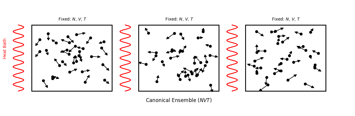
We start by considering an islolated box ( $NVE$ ensemble) inside which there is a system of interest which is exchanging energy with much larger reserovoir or heat bath.
Using the fact that reservoir is much larger than the system $E \ll E_t$ we can taylor expand log of microstates (entropy) around $E_t$

p(E) = \frac{\Omega(E) \Omega_r(E_t - E)}{\Omega_t(E_t)}

(38)

log\Omega_r(E_t-E) \approx log\Omega_r(E_t) - \bigg(\frac{\partial log \Omega_r}{\partial E} \bigg) E = const - \beta E

(39)

The first factor is a constant independent of energy the second factor in front of energy is recognize as inverse temperature $\beta = \frac{dlog\Omega}{dE}=\frac{1}{k_BT}$
We have now have an ensemble of microstates of systems specified by $NVT$ variables and and reservoir influence enters through temperature!
Ensemble of $NVT$ microstates has different energies that are exponentially distributed (price for borrowing energy from the bath).

\Omega_r(E_t - E) \sim e^{- \beta E}

(40)

MaxEnt leads to canonical distribution

We can use Maximizing Entropy principle to assing probabilities for an esnemble where we have a physical constraint placed on having fixed average energy $\langle E\rangle =U$

J[p_i] = \sum -p_ilog p_i -\alpha \bigg(\sum_i-1 \bigg)-\beta \bigg(\sum_i p_i E_i -U \bigg)

(44)

\delta J = 0 \rightarrow -1 -logp_i -\alpha-\beta p_i=0

(45)

Probability of each microstate is now weighted by an exponential of microstate Energies:

p_i = \frac{e^{-\beta E_i}}{\sum_i e^{-\beta E_i}}

(46)

Probability of each macrostate containing $\Omega(E)$ number of microstates would be:

p(E) = \frac{\Omega(E)e^{-\beta E}}{\sum_E \Omega(E) e^{-\beta E}}

(47)

By comparing with thermodynamics we can confirm that lagrange coefficinet is inverse temperature $\beta=\frac{1}{k_BT}$

Partition Functions and Thermodynamic limit¶

Z = \sum_E \Omega(E) e^{-\beta E} = \int \sum \Omega(E) e^{-\beta E} dE

(48)

We find that microcanonical and canonical ensebles are linked via Laplace transform. Recall that $E$ and free energy $F$ via Legendre transform
This shows that when going from $NVE$ to $NVT$ ensemble we are adopting a conveneint variable $\beta$ by replacing $E$ .
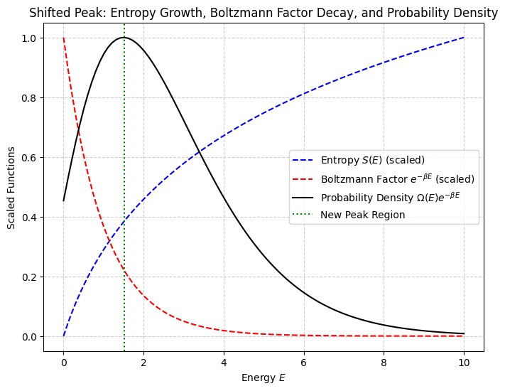
The number of states grows exponentially with system size $N$ , $\Omega(E) = e^{\frac{S}{k_B}} \sim e^{N}$ while the Boltzmann factor decays exponentially with energy $e^{-\beta E} \sim e^{-N}$
The dominant contribution to the partition function comes from narrow region around ensemble average or equilibrium value of energy $U=\langle E\rangle$ . Deviations from average are xponentially negligble!

import numpy as np
import matplotlib.pyplot as plt

# Define energy range
E = np.linspace(0, 10, 100)

# Define parameters
beta = 1.0  # Inverse temperature (1/kT)

# Compute the Boltzmann factor
Boltzmann_factor = np.exp(-beta * E)

# Increase the entropy prefactor to shift the peak to the right
S_prefactor_new = 2.5  # Larger prefactor makes entropy increase faster

# Recalculate entropy and probability density
S_new = S_prefactor_new * np.log(1 + E)
Probability_density_new = np.exp(S_new) * Boltzmann_factor

# Create the updated plot
plt.figure(figsize=(8, 6))

# Plot entropy (scaled for visualization)
plt.plot(E, S_new / max(S_new), label=r"Entropy $S(E)$ (scaled)", color="blue", linestyle="--")

# Plot Boltzmann factor (scaled for visualization)
plt.plot(E, Boltzmann_factor / max(Boltzmann_factor), label=r"Boltzmann Factor $e^{-\beta E}$ (scaled)", color="red", linestyle="--")

# Plot updated probability density (product of both)
plt.plot(E, Probability_density_new / max(Probability_density_new), label=r"Probability Density $\Omega(E) e^{-\beta E}$", color="black")

# Highlight new peak region
E_peak_new = E[np.argmax(Probability_density_new)]
plt.axvline(E_peak_new, color="green", linestyle=":", label="New Peak Region")

# Labels and title
plt.xlabel("Energy $E$")
plt.ylabel("Scaled Functions")
plt.title("Shifted Peak: Entropy Growth, Boltzmann Factor Decay, and Probability Density")
plt.legend()
plt.grid(True, linestyle="--", alpha=0.6)

# Show plot
plt.show()

Examples of using NVT¶

non-interacting spins¶

Consider an ensemble of three non-interaacting spins under constant temperature. The up spin has $\epsilon$ and down spin 0 energy.

Microstate	Configuration	Total Energy $E$	Degeneracy $\Omega(E)$
1	$\downarrow \downarrow \downarrow$	0	1
2	$\downarrow \downarrow \uparrow$	$\epsilon$	3
3	$\downarrow \uparrow \downarrow$	$\epsilon$	3
4	$\uparrow \downarrow \downarrow$	$\epsilon$	3
5	$\downarrow \uparrow \uparrow$	$2\epsilon$	3
6	$\uparrow \downarrow \uparrow$	$2\epsilon$	3
7	$\uparrow \uparrow \downarrow$	$2\epsilon$	3
8	$\uparrow \uparrow \uparrow$	$3\epsilon$	1

The partition function would be sum over all $2^3=8$ microstaes.

Z = 1+3e^{-\beta \epsilon}+ 3e^{-2\beta \epsilon}+e^{-3\beta \epsilon}

(51)

Probability of a microstate $\downarrow \downarrow \uparrow$ is:

p_2 = \frac{e^{-\beta \epsilon}}{Z}

(52)

Probability of a macrostate $E=\epsilon$ is

P(E=\epsilon) = \frac{3e^{-\beta \epsilon}}{Z}

(53)

non-interacting indentical spins

Consider three spins where up and down orientations have equal energy $\epsilon$ .
Show that sum over microstates and sum over macrostates leads to same expression of parition function.
Write down free energy for the system and identify entropic and energetic parts.

Two-state particles (NVT)¶

Consider a simple two-level system where lower level has energy 0 and upper level $\epsilon$ . Determine how the fraction of excited states $f=\frac{n}{N}$ changes with temperature.
Solving a two-state particle system in an NVT ensemble is much easier because the partition function decouples into single particle contributions.

Z = \sum^{n=N}_{n=0} e^{-\beta E_n} = (1+e^{-\beta \epsilon})^N

(60)

F= -k_B T log Z = -k_BT N log(1+e^{-\beta \epsilon})

(61)

\langle E \rangle = \frac{\partial log Z}{\partial (-\beta)} = \frac{N\epsilon}{1+e^{\beta \epsilon}}

(62)

f = \frac{E}{N\epsilon} = \frac{1}{1+e^{\beta \epsilon}}

(63)

We obtained same expression we got when using NVE but it tooks us less number of steps!

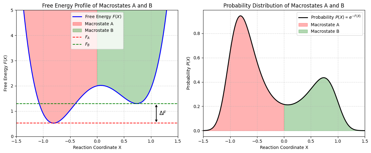
Free energy and macrostate probabilities¶

Microstates: The relative population of microstates is dictated by the ratio of Boltzmann weights which depends on energy difference $\Delta E$

p_1 = \frac{e^{-\beta E_1}}{Z} = \frac{e^{-\beta E_1}}{e^{-\beta F}}

(64)

{\frac{p_2}{p_1} = e^{-\beta (E_2-E_1)}}

(65)

Macrostates: Probability of macrostates with energy $E_A$ is obtained by summing over all microstates with energy E_A or simply by multiplying by $\Omega_A$ . The latter is related to entropy, which ends up turning the numerator into the free energy of a macrostate $A$ : $F_A = E_A-TS_A$

p_A =\frac{\Omega (E_A) e^{-\beta E_A}}{Z_A} = \frac{e^{-\beta F_A}}{e^{-\beta F}}

(66)

The relative population of macrostates is dictated by the ratio of entropic term times Boltzmann weights which depends on free energy difference $\Delta F$

{\frac{p_B}{p_A} = e^{-\beta (F_B-F_A)}}

(67)

# Define reaction coordinate
import numpy as np
import matplotlib.pyplot as plt

x = np.linspace(-2, 2, 400)

# Define a tilted asymmetric double-well free energy profile
F_x = 3 * (x**4 - 1.2*x**2) + 2 + 0.5*x  # Added tilt to shift one minimum

# Identify macrostates A and B based on regions left and right of the transition state (x=0)
x_A_region = x[x < 0]  # Left basin (macrostate A)
x_B_region = x[x > 0]  # Right basin (macrostate B)
F_A = np.min(F_x[x < 0])  # Free energy of macrostate A (left well minimum)
F_B = np.min(F_x[x > 0])  # Free energy of macrostate B (right well minimum)
ΔF = F_B - F_A  # Free energy difference

# Compute probability distribution P(X) from free energy F(X)
P_x = np.exp(-F_x)  # Exponential of negative free energy
P_x /= np.trapz(P_x, x)  # Normalize probability

# Create figure with side-by-side subplots: Free Energy and Probability Distribution
fig, axes = plt.subplots(1, 2, figsize=(12, 5), sharex=True)

# --- Free Energy Profile ---
axes[0].plot(x, F_x, label=r'Free Energy $F(X)$', color='b', linewidth=2)
axes[0].fill_between(x_A_region, F_x[x < 0], max(F_x), color='red', alpha=0.3, label="Macrostate A")
axes[0].fill_between(x_B_region, F_x[x > 0], max(F_x), color='green', alpha=0.3, label="Macrostate B")
axes[0].axhline(F_A, color='red', linestyle='--', label=r'$F_A$')
axes[0].axhline(F_B, color='green', linestyle='--', label=r'$F_B$')

# Indicate ΔF with an arrow
axes[0].annotate("", xy=(1.1, F_B), xytext=(1.1, F_A),
                 arrowprops=dict(arrowstyle="<->", color='black', linewidth=1.5))
axes[0].text(1.15, (F_A + F_B) / 2, r'$\Delta F$', va='center', fontsize=12, color='black')

axes[0].set_xlabel("Reaction Coordinate X")
axes[0].set_ylabel("Free Energy $F(X)$")
axes[0].set_title("Free Energy Profile of Macrostates A and B")
axes[0].legend()
axes[0].grid(True, linestyle="--", alpha=0.5)
axes[0].set_xlim([-1.5, 1.5])
axes[0].set_ylim([0, 5])

# --- Probability Distribution ---
axes[1].plot(x, P_x, label=r'Probability $P(X) \propto e^{-F(X)}$', color='black', linewidth=2)
axes[1].fill_between(x_A_region, P_x[x < 0], 0, color='red', alpha=0.3, label="Macrostate A")
axes[1].fill_between(x_B_region, P_x[x > 0], 0, color='green', alpha=0.3, label="Macrostate B")

axes[1].set_xlabel("Reaction Coordinate X")
axes[1].set_ylabel("Probability $P(X)$")
axes[1].set_title("Probability Distribution of Macrostates A and B")
axes[1].legend()
axes[1].grid(True, linestyle="--", alpha=0.5)

# Adjust layout and show the plots
plt.tight_layout()
plt.show()

---------------------------------------------------------------------------
AttributeError                            Traceback (most recent call last)
Cell In[10], line 19
     17 # Compute probability distribution P(X) from free energy F(X)
     18 P_x = np.exp(-F_x)  # Exponential of negative free energy
---> 19 P_x /= np.trapz(P_x, x)  # Normalize probability
     21 # Create figure with side-by-side subplots: Free Energy and Probability Distribution
     22 fig, axes = plt.subplots(1, 2, figsize=(12, 5), sharex=True)

File /opt/hostedtoolcache/Python/3.12.12/x64/lib/python3.12/site-packages/numpy/__init__.py:792, in __getattr__(attr)
    789     import numpy.char as char
    790     return char.chararray
--> 792 raise AttributeError(f"module {__name__!r} has no attribute {attr!r}")

AttributeError: module 'numpy' has no attribute 'trapz'

Energy Fluctuations¶

Log of canonical parition function $logZ$ has some interesting mathematical properties.
We are going to show that first and second derivatives yield average and fluctuations of energy.

P_i = \frac{e^{-\beta E_i}}{Z}, \quad Z = \sum_i e^{-\beta E_i}

(69)

The ensemble average energy can be related to the derivative of log of partition function:

\langle E \rangle = \sum_i P_i E_i = \frac{1}{Z} \sum_i E_i e^{-\beta E_i} = -\frac{1}{Z} \frac{\partial Z}{\partial \beta} = -\frac{\partial \ln Z}{\partial \beta}

(70)

To quantify fluctuations, we define the variance of energy and proceed to show that this is equal to second erivative of logZ

\langle (\Delta E)^2 \rangle = \langle E^2 \rangle - \langle E \rangle^2

(71)

Taking first derivative:

\frac{\partial \ln Z}{\partial \beta} = -\frac{1}{Z} \sum_i E_i e^{-\beta E_i} = -\langle E \rangle

(72)

Taking the second derivative:

\frac{\partial^2 \ln Z}{\partial \beta^2} = \frac{1}{Z} \sum_i E_i^2 e^{-\beta E_i} - \left(\frac{1}{Z} \sum_i E_i e^{-\beta E_i} \right)^2

(73)

\frac{\partial^2 \ln Z}{\partial \beta^2} = \langle E^2 \rangle - \langle E \rangle^2 = \langle (\Delta E)^2 \rangle

(74)

Since $\beta = \frac{1}{k_B T}$ , we can use chain rule and express this in terms of temperature:

\langle (\Delta E)^2 \rangle = k_B T^2 \frac{\partial \langle E \rangle}{\partial T} = k_B T^2C_v

(75)

Where in the last line we used definition of heat capacity $C_V = \frac{d\langle E\rangle}{dT}$

The probability distribution of energy, $P(E)$ , follows a Gaussian distribution in equilibrium:
$P(E) \propto \exp\left(-\frac{(E - \langle E \rangle)^2}{2 k_B T^2 C_V} \right)$
(79)
Relative energy fluctuations decrease with $N$ . In the thermodynamic limit $N\rightarrow \infty$ , fluctuations become negligible, justifying ensemble equivalence.
$\frac{\sigma_E}{\langle E \rangle} \sim \frac{C_V^{1/2}}{\langle E \rangle} \sim O(N^{-1/2})$
(80)

Statistical nature of irreversibility¶

From the perspective of the NVE ensemble, we can state that if the number of accessible microstates increases upon the removal of a constraint, then reinstating the constraint will not spontaneously reduce it. This reflects the fundamental irreversibility of spontaneous processes in an isolated system:

\Delta S = \log \frac{\Omega_{B}}{\Omega_{A}} \geq 0.

(81)

A similar conclusion holds in the NVT ensemble: Under constant temperature, the number of microstates, represented by the partition function $Z$ , increases during a spontaneous process when a system is in contact with a heat bath.
$-\beta \Delta F = \log \frac{Z_{B}}{Z_{A}} \geq 0.$
(82)
This formulation underscores the irreversibility of thermodynamic processes and highlights the natural tendency of a system to evolve towards configurations with higher entropy (in the microcanonical ensemble) or lower free energy (in the canonical ensemble).

Problems¶

Problem 1 Shottky defects¶

Schotky defects are vacancies in a lattice of atoms. Creating a single vacancy costs an energy $\epsilon$ . Consider a lattice with $N$ atoms and $n$ vacacnies. In this model the total energy is solely a function of defects: $E=n\epsilon$

Write down number of states and compute the entropy via Boltzmann formula. Plot number of states as a function of energy. You can use log of number of states for plotting.
Compute how the temperature would affect the fraction of vacancies on the lattice. Plot fraction of vacancies as a function of temperature.
How would the total energy depend on temperature $T$ . Derive expression for the high temeprature limit ( $\frac{\epsilon}{k_b T} \gg 1$ ).
Plot total energy as a function of temperature E(T)

Problem 2 Lattice gas¶

Consider $N$ particles distributed among $V$ cells (with $N\ll V$ ). This is a lattice model of a dilute gas. Suppose that each cell may be either empty or occupied by a single particle. The number of microscopic states of this syste will be given by:

\Omega (N, V) = \frac{V!}{N! (V-N)!}

(83)

Obtain an expression for the entropy per particle $s(v)=\frac{1}{N} \cdot S(N,V)$ where $v=\frac{V}{N}$ .
From this simple fundamental equation, obtain an expression of equation of state $p/T$ .
- Write an expansion of $p/T$ in terms of density $1/v$ . Show that the first term gives Boyle law of ideal gases.
Sketch a graph of $\mu/T$ , where $\mu(\rho)$ is a chemical potential as a function of density. Comment on $\rho\rightarrow 0$ and $\rho\rightarrow 1$ limits.

Problem 3 Polymer Elasticity¶

Solve the problem 2.7 from the book.

Problem 4¶

Consider a system of N classical and non-interacting particles in contact with a thermal reservoir at a temperature $T$ . Each particle can have be in three states with energy 0, $\epsilon$ or $3\epsilon$ where $\epsilon>0$ .

Obtain an expression for $Z$ then compute the average and fluctuation of energy.
Plot the heat capacity as a function of temperature $C_v(T)$
Plot the average enegy as a function of temperature $U(T)$
Plot the entropy as a function of temperature $S(T)$ .

Problem 5¶

Consider $N$ lattice sites which have quantum spins $s=1$ (not to be confused with entropy) with a mangnetic moment $\mu$ . Spins are subject to a uniform mangeitc field in z direction $B=B_z$ making the energy of each spin $-\mu B m$ where $m$ is the magnetic quantum number thattakes on three possible values $m=0, \pm 1$ .

Compute the entropy $S$ and the mangeitzation of the system $M$
Plot entropy as a function of temperatures and study the limit of low temperatures $S(T\rightarrow 0)$