Ensembles in phase-space

Quantization of Phase Space in Units of $h$ ¶

figure-md - Unknown Directive

<img src="./figs/1d-pspace.png" class="bg-primary" width="300px">  

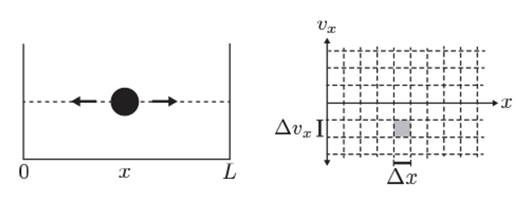
Illustration of phase space for a 1D particle in a box.

In classical mechanics, a system’s state is represented as a point in phase space, with coordinates $(x, p)$ for each degree of freedom. The number of microstates is, in principle, infinite because both position and momentum can vary continuously.
However, in quantum mechanics, the Heisenberg uncertainty principle imposes a fundamental limit on how precisely position and momentum can be specified:
This implies that we cannot resolve phase space with arbitrary precision. Instead, each distinguishable quantum state occupies a minimum phase space volume on the order of:

\Delta x \, \Delta p \sim h

(1)

For a system with $f$ degrees of freedom (e.g $3N$ for $N$ particles in three dimensions), the smallest resolvable cell in phase space has volume:

(\Delta x \, \Delta p)^f \sim h^f

(2)

To compute the number of accessible microstates $\Omega$ in a given region of phase space, we divide the classical phase space volume $\Gamma$ by the smallest quantum volume $h^f$
Since N particles are indistingusihable and classical mechanics has no such concept we have to manually divide numer of microstates by $N!$

\Omega(E) = \frac{\Gamma}{h^f N!}

(3)

An explicit expression for number of microstates for a given energy $E$ is written by using delta function which counts all microstates in phase-space where $H(p^N, x^N)=E$

Phase-space of a harmonic oscillator

H(x, p) = \frac{p^2}{2m} + \frac{1}{2} m \omega^2 x^2

(5)

$x$ = position, $p$ = momentum, $m$ = mass, $\omega$ = angular frequency
This Hamiltonian gives the total energy $E$ of a particle undergoing simple harmonic motion.
Setting $H(x, p) = E$ , we get the constant-energy curve:

\frac{x^2}{\left( \sqrt{\frac{2E}{m \omega^2}} \right)^2} + \frac{p^2}{\left( \sqrt{2mE} \right)^2} = 1

(6)

This is the equation of an ellipse in the $(x, p)$ phase space, with:
- Semi-major axis: $a = \sqrt{\frac{2E}{m \omega^2}}$ (in $x$ )
- Semi-minor axis: $b = \sqrt{2mE}$ (in $p$ )

Compute Area of the Ellipse (Classical Action)

A = \pi a b = \pi \sqrt{\frac{2E}{m \omega^2}} \cdot \sqrt{2mE} = \frac{2\pi E}{\omega}

(7)

Plugging in quantum mechanical expression of quantized energies of harmonic oscillator

E= \hbar\omega\bigg(n+\frac{1}{2} \bigg)

(8)

This area corresponds to the classical action integral $\oint p \, dx$ , which in semiclassical quantization becomes:

\oint p \, dx = (n + \tfrac{1}{2}) h

(9)

import numpy as np
import matplotlib.pyplot as plt

# Set constants
hbar = 1.0
h = 2 * np.pi * hbar
m = 1.0
omega = 1.0

# Quantum numbers to plot
n_values = [0, 1, 2, 5, 10]

# Prepare plot
fig, ax = plt.subplots(figsize=(5, 4))

# Colors for each energy level
colors = plt.cm.viridis(np.linspace(0, 1, len(n_values)))

# Store areas for demonstration
areas = []

# Plot ellipses for each energy level
for i, n in enumerate(n_values):
    E_n = hbar * omega * (n + 0.5)
    a = np.sqrt(2 * E_n / (m * omega**2))  # x_max
    b = np.sqrt(2 * m * E_n)               # p_max
    theta = np.linspace(0, 2 * np.pi, 500)
    x = a * np.cos(theta)
    p = b * np.sin(theta)
    ax.plot(x, p, label=f"n = {n}", color=colors[i])
    
    # Area of ellipse = πab (quasi-classical action)
    A_n = np.pi * a * b
    areas.append((n, A_n / h))  # normalized by h

# Annotate areas
for n, A_h in areas:
    ax.text(0.1, 1.1 * np.sqrt(2 * m * hbar * omega * (n + 0.5)), 
            f"$A/h$ ≈ {A_h:.1f}", fontsize=9)

# Final plot settings
ax.set_xlabel("Position $x$")
ax.set_ylabel("Momentum $p$")
ax.set_title("Harmonic Oscillator Phase Space: Quasi-Classical Area $\oint p \\, dx$")
ax.set_aspect('equal')
ax.legend()
ax.grid(True)

plt.tight_layout()
plt.show()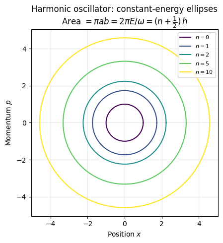

<>:44: SyntaxWarning: invalid escape sequence '\o'
<>:44: SyntaxWarning: invalid escape sequence '\o'
/tmp/ipykernel_2876/746595933.py:44: SyntaxWarning: invalid escape sequence '\o'
  ax.set_title("Harmonic Oscillator Phase Space: Quasi-Classical Area $\oint p \\, dx$")

Computing Z via classical mechanics¶

In quantum mechanics counting microsites is easy, we have discrete energies and could simply sum over microstates to compute partition functions

Z=\sum_i e^{-\beta E_i}

(10)

Counting microstates in classical mechanics is therefore done by discretizing phase space for N particle system $x^N, p^N$ into smallest unit boxes of size $h^N$ .

\sum_i \rightarrow \int \frac{dpdx}{h}

(11)

Once agan to correct classical mechanics for “double counting” of microstates if we have N indistinguishable “particles” with a factor of $N!$

The power and utility of NVT: The non-interacting system¶

For the independent particle system, the energy of each particle enter the total energy of the system additively.

E(\epsilon_1, \epsilon_2, ... \epsilon_N) = \epsilon_1+\epsilon_2+...\epsilon_N

(13)

The exponential factor in the partition function allows decoupling particle contributions $e^{-\beta{(\epsilon_1+\epsilon_2)}} = e^{-\beta{\epsilon_1}}e^{-\beta{\epsilon_2}}$ . This means that the partition function can be written as the product of the partition functions of individual particles!

Distinguishable states:

Z = z_1 \cdot z_2 \cdot z_3 ... z_N

(14)

Indistinguishable states:

Z = \frac{1}{N!}z^N

(15)

Maxwell-Boltzman distribution¶

Since the kinetic and potential energy functions depend separately on momenta and positions, the total probability distribution factorizes into a product of position and momentum distributions:

H(p^N, r^N) = U(r^N) + K(p^N) = U(r^N) + \sum_{i=1}^{N} \frac{p_i^2}{2m}

(16)

This separation leads to:

P(r^N, p^N) = P(r^N) \cdot P(p^N) = \int_V dr^N \, e^{-\beta U(r^N)} \cdot \int_{-\infty}^{+\infty} dp^N \, e^{-\beta \sum_{i=1}^{N} \frac{p_i^2}{2m}}

(17)

The intergarlwith position-dependent potential for interacting particle system is impossible to evaluate except by simulations or numerical techniques
The momentum-dependent part splits into individaul integrals for every particle and is always a simple quadratic function, making it analytically tractable:

P(p^N) = \left[ \int_{-\infty}^{+\infty} dp \, e^{-\beta \frac{p^2}{2m}} \right]^N

(18)

The momentum (or velocity) distribution follows the Maxwell-Boltzmann distribution in all equilibrium systems, regardless of the complexity of the molecular interactions.

Maxwell-Boltzmann Velocity Distribution: Full Derivation

Separation of variables

In equilibrium, the distribution of velocities in the $x$ , $y$ , and $z$ directions are independent and identical, because there’s no preferred direction in an ideal gas. Therefore, we can write the joint probability distribution as:

f(v_x, v_y, v_z) = f(v_x)f(v_y)f(v_z)

(19)

Furthermore, the probability of finding a particle with velocity components between $(v_x, v_x + dv_x)$ , $(v_y, v_y + dv_y)$ , and $(v_z, v_z + dv_z)$ is:

f(v_x, v_y, v_z) dv_x dv_y dv_z

(20)

Form of the velocity component distribution

The system is in thermal equilibrium, so the probability of a particle having a certain velocity corresponds to the Boltzmann factor for its kinetic energy:

\text{Probability} \propto e^{-E_{\text{kin}} / k_B T}

(21)

For a single particle of mass $m$ , the kinetic energy is:

E_{\text{kin}} = \frac{1}{2}m(v_x^2 + v_y^2 + v_z^2)

(22)

So we postulate:

f(v_x, v_y, v_z) \propto e^{-m(v_x^2 + v_y^2 + v_z^2)/2k_B T}

(23)

Using the independence of the components:

f(v_x) \propto e^{- m v_x^2 / 2 k_B T}

(24)

We require that:

\int_{-\infty}^\infty f(v_x) dv_x = 1

(25)

This is a standard Gaussian integral of form $p(x) = \frac{1}{\sqrt{2\pi \sigma^2}} e^{-\frac{x^2}{2\sigma^2}}$ where $\sigma^2 = \frac{k_B T}{m}$ and therefore we write down:

f(v_x) = \sqrt{\frac{m}{2\pi k_B T}} \, e^{- \frac{1}{2} m v_x^2 / k_B T}

(26)

Distribution of speeds

Now, let’s consider the speed $v = \sqrt{v_x^2 + v_y^2 + v_z^2}$ .
The probability density for the speed (regardless of direction) is obtained by converting to spherical coordinates in velocity space. The volume element in velocity space becomes:

dv_x dv_y dv_z = v^2 \sin\theta \, dv \, d\theta \, d\phi

(27)

Integrating over angles gives a factor of $4\pi$ :

f(v) dv = \underbrace{4\pi v^2}_{\text{Jacobian}} \cdot f(v_x)f(v_y)f(v_z) dv

(28)

Substitute in the expressions for $f(v_x)$ , $f(v_y)$ , and $f(v_z)$ , and recall that the total exponent is:

f(v_x)f(v_y)f(v_z) = \left(\frac{m}{2\pi k_B T}\right)^{3/2} e^{-\frac{1}{2} m (v_x^2 + v_y^2 + v_z^2) / k_B T} = \left(\frac{m}{2\pi k_B T}\right)^{3/2} e^{- \frac{1}{2} m v^2 / k_B T}

(29)

Therefore, the speed distribution is:

f(v) = 4\pi v^2 \left( \frac{m}{2\pi k_B T} \right)^{3/2} e^{- \frac{1}{2} m v^2 / k_B T}

(30)

This is the Maxwell-Boltzmann speed distribution. It gives the probability density that a particle in a gas has speed $v$ .

import numpy as np
import matplotlib.pyplot as plt

# Constants for Maxwell-Boltzmann Distribution (in arbitrary units)
k_B = 1.38e-23   # Boltzmann constant (J/K), not used directly since we'll use reduced units
T = 300          # Temperature in K
m = 4.65e-26     # Mass of nitrogen molecule (kg), approximate

# Define velocity range
v = np.linspace(0, 2000, 1000)

# Maxwell-Boltzmann distribution function
def f_MB(v, m, T):
    return 4 * np.pi * v**2 * (m / (2 * np.pi * k_B * T))**(3/2) * np.exp(-m * v**2 / (2 * k_B * T))

# Compute distribution
f_v = f_MB(v, m, T)

# Characteristic velocities
v_mp = np.sqrt(2 * k_B * T / m)         # Most probable speed
v_avg = np.sqrt(8 * k_B * T / (np.pi * m))  # Average speed
v_rms = np.sqrt(3 * k_B * T / m)        # Root mean square speed

# Plot
plt.figure(figsize=(10, 6))
plt.plot(v, f_v, label="Maxwell-Boltzmann Distribution", color='black')
plt.axvline(v_mp, color='blue', linestyle='--', label=f"$v_{{\\rm mp}}$ = {v_mp:.0f} m/s")
plt.axvline(v_avg, color='green', linestyle='--', label=f"$\\langle v \\rangle$ = {v_avg:.0f} m/s")
plt.axvline(v_rms, color='red', linestyle='--', label=f"$v_{{\\rm rms}}$ = {v_rms:.0f} m/s")
plt.title("Maxwell-Boltzmann Speed Distribution for $N_2$ at 300 K")
plt.xlabel("Speed (m/s)")
plt.ylabel("Probability Density")
plt.legend()
plt.grid(True)
plt.tight_layout()
plt.show()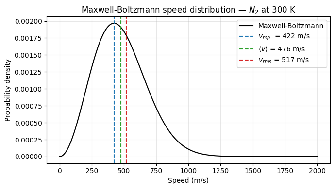

Ideal Gas¶

A useful approximation is to consider the limit of a very dilute gas, known as an ideal gas, where interactions between particles are neglected $V = 0$ .
Lets evaluate partition function for a single atom of idea gas:

z(\beta) = \left[ \frac{1}{h} \int_{0}^{L} dx \int_{-\infty}^{+\infty} dp \, e^{- \frac{p^2}{2m k_B T}} \right]^3 = V \left( \frac{2\pi m k_B T}{h^2 } \right)^{3/2}

(33)

z = \frac{V}{\lambda^3_T} = V n_Q

(34)

On the Validity of the Classical Approximation

The classical approximation is valid when the average interatomic spacing $\sim n^{-1/3}$ is much larger than $\lambda_T$ , i.e., when:

n \lambda_T^3 \ll 1

(37)

This ensures that wavefunction overlap is negligible and particles behave classically.

We can also calculate entropy and other thermodynamic quantities and compare with expressions obtained in $NVE$ ensemble

S = -\Big( \frac{\partial F}{\partial T}\Big)_{N,V} = Nk_B \Bigg[log \Big( \frac{n_Q}{n} \Big)+ \frac{5}{2} \Bigg]

(41)

U = \frac{\partial log Z}{\partial (-\beta)} = \frac{3}{2}N k_B T

(42)

p = -\frac{\partial F}{\partial V} =\frac{N k_B T}{V}

(43)

Equipartition Theorem¶

Consider a classical system with a Hamiltonian containing a quadratic degree of freedom $x$ , such that:

E(x) = \frac{1}{2} a x^2

(44)

The canonical partition function for this degree of freedom is:

Z = \int_{-\infty}^{\infty} e^{-\beta \frac{1}{2} a x^2} dx = \sqrt{\frac{2\pi}{\beta a}}

(45)

The average energy is:

\langle E \rangle = -\frac{\partial \log Z}{\partial \beta}

(46)

\log Z = \frac{1}{2} \log \left( \frac{2\pi}{\beta a} \right) = \text{const} - \frac{1}{2} \log \beta

(47)

\langle E \rangle = -\frac{\partial}{\partial \beta} \left( -\frac{1}{2} \log \beta \right) = \frac{1}{2\beta} = \frac{1}{2} k_B T

(48)

Examples¶

Monatomic ideal gas: 3 translational degrees → $\langle E \rangle = \frac{3}{2} k_B T$
Diatomic molecule at high $T$ : 3 translational + 2 rotational + $n$ active vibrational modes
→ $\langle E \rangle = \left( \frac{5}{2} + n \right) k_B T$

Partition functions for non-interacting molecules¶

Total energy and partition function for a molecule with separable degrees of freedom:

Translational Degrees of Freedom: Particle in a Box¶

For a particle in a 3D box of volume $V = L^3$ , the energy levels are:

E_{n_x, n_y, n_z} = \frac{\hbar^2 \pi^2}{2m L^2} \left(n_x^2 + n_y^2 + n_z^2 \right)

(52)

To approximate the partition function at high temperatures (many levels populated), we replace the discrete sum with an integral:

Z = \sum_{n_x, n_y, n_z} e^{-\beta E_{n_x, n_y, n_z}} \approx \left[ \int_0^\infty dn\, e^{-\beta \frac{\hbar^2 \pi^2}{2m L^2} n^2} \right]^3

(53)

This is a Gaussian integral:

\int_0^\infty e^{-a n^2} dn = \frac{1}{2} \sqrt{\frac{\pi}{a}}

(54)

Z = \left[ \frac{1}{2} \sqrt{\frac{\pi}{\frac{\hbar^2 \pi^2}{2m L^2} \beta}} \right]^3 = \left( \frac{L}{h} \sqrt{2 \pi m k_B T} \right)^3 = V \left( \frac{m k_B T}{2\pi \hbar^2} \right)^{3/2} = V n_Q

(55)

For $N$ indistinguishable molecules we obtain same result we go for ideal gas!

Z = \frac{(V n_Q)^N}{N!}

(56)

Rotational Degrees of Freedom: Rigid Rotor Model¶

For a linear molecule (diatomic rotor), the rotational energy levels are:

E_J = \frac{\hbar^2}{2I} J(J + 1), \quad \text{with degeneracy } (2J + 1)

(57)

The partition function is:

Z = \sum_{J=0}^\infty (2J + 1) e^{-\beta \frac{\hbar^2}{2I} J(J + 1)}

(58)

At high temperatures ( $k_B T \gg \hbar^2 / 2I$ ), this sum can be approximated as an integral:

Z \approx \int_0^\infty (2J + 1)\, e^{-\beta \frac{\hbar^2}{2I} J(J + 1)}\, dJ

(59)

Let $x = J(J+1) \approx J^2$ for large $J$ :

Z \approx \int_0^\infty 2J\, e^{-\beta \frac{\hbar^2}{2I} J^2}\, dJ

(60)

This integral is:

\int_0^\infty J e^{-a J^2} dJ = \frac{1}{2a}

(61)

Z \approx \frac{1}{\beta \frac{\hbar^2}{2I}} = \frac{2I k_B T}{\hbar^2} = \frac{T}{\theta_{\text{rot}}}

(62)

Where $\theta_{\text{rot}} = \frac{\hbar^2}{2I k_B}$ is the rotational temperature.

Vibrational Degrees of Freedom: Harmonic Oscillator Model¶

E_n = \hbar \omega \left(n + \frac{1}{2}\right)

(63)

Partition function for one oscillator:

z = \sum_{n=0}^\infty e^{-\beta \hbar \omega (n + \frac{1}{2})} = e^{-\frac{1}{2} \beta \hbar \omega} \sum_{n=0}^\infty \left(e^{-\beta \hbar \omega}\right)^n = \frac{e^{-\frac{1}{2} \beta \hbar \omega}}{1 - e^{-\beta \hbar \omega}}

(64)

For $N$ independent oscillators:

Z = z^N

(65)

Average energy would then be:

E = -\frac{\partial \log Z}{\partial \beta} = -N \frac{\partial \log z}{\partial \beta}

(66)

\log z = -\frac{1}{2} \beta \hbar \omega - \log\left(1 - e^{-\beta \hbar \omega} \right)

(67)

\frac{\partial \log z}{\partial \beta} = -\frac{1}{2} \hbar \omega + \frac{\hbar \omega\, e^{-\beta \hbar \omega}}{1 - e^{-\beta \hbar \omega}} = -\frac{1}{2} \hbar \omega + \frac{\hbar \omega}{e^{\beta \hbar \omega} - 1}

(68)

E = N \hbar \omega \left( \frac{1}{2} + \frac{1}{e^{\beta \hbar \omega} - 1} \right)

(69)

Low and high temperature behaviours of harmonic oscillators¶

Notice the two important limits. At low temperature quantization of energy becomes important while at high temperature result matches with classical mechanics predictions;
As $T \rightarrow 0$ , $e^{\beta \hbar \omega} \gg 1$ , so:

E \rightarrow N \cdot \frac{1}{2} \hbar \omega

(70)

As $T \rightarrow \infty$ , $e^{\beta \hbar \omega} \approx 1 + \beta \hbar \omega$ :

\frac{1}{e^{\beta \hbar \omega} - 1} \approx \frac{1}{\beta \hbar \omega} \Rightarrow E \approx N k_B T

(71)

# Temperature range in Kelvin
T_vals = np.linspace(10, 5000, 500)

# Vibrational frequency (typical for molecular vibration)
# Use hbar*omega = energy quantum = ~0.2 eV (~3200 cm^-1 IR band), convert to J
hbar_omega = 0.2 * 1.602e-19  # in J

# Dimensionless variable x = hbar*omega / (k_B * T)
x = hbar_omega / (k_B * T_vals)

# Heat capacity C_v of harmonic oscillator (per mode)
# C_v = k_B * (x^2 * exp(x)) / (exp(x) - 1)^2
C_v = k_B * (x**2 * np.exp(x)) / (np.exp(x) - 1)**2

# Convert C_v to units of k_B
C_v_over_kB = C_v / k_B

# Plot
plt.figure(figsize=(8, 5))
plt.plot(T_vals, C_v_over_kB, color='darkorange')
plt.xlabel("Temperature (K)")
plt.ylabel("Heat Capacity $C_V / k_B$")
plt.title("Heat Capacity of a Quantum Harmonic Oscillator vs Temperature")
plt.grid(True)
plt.tight_layout()
plt.show()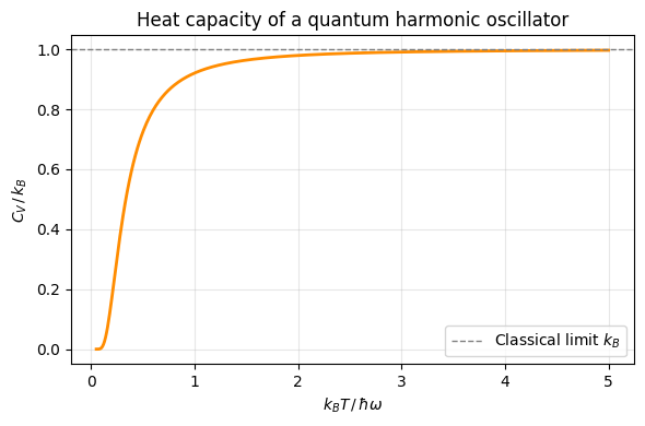

On heat capacity of harmonic-oscillators¶

Einstein Model of solids¶

A simple model for solids due to Einstein describes it as $N$ independent harmonic oscillators representing localized atomic vibrations.
The average energy of a quantum harmonic oscillator is:

\langle E \rangle = \hbar \omega \left( \frac{1}{2} + \frac{1}{e^{\beta \hbar \omega} - 1} \right)

(72)

The heat capacity is the derivative:

C_V = \frac{\partial \langle E \rangle}{\partial T} = k_B \left( \frac{x^2 e^x}{(e^x - 1)^2} \right), \quad x = \frac{\hbar \omega}{k_B T}

(73)

Key predictions of Einstein model of solids¶

At low T: $C_V \to 0$ — the oscillator is frozen in its ground state.
At high T: $C_V \to k_B$ — classical equipartition is recovered.

Debye Model of Solids¶

The Debye model improves upon Einstein’s and matches experimental data much better than the Einstein model, especially at low temperatures.
Main distinguishing features of Debye model are:
- Treating atomic vibrations as a continuum of phonon modes.
- Including a full spectrum of frequencies up to a Debye cutoff $\omega_D$ .
- Predicting the correct low-temperature behavior of solids.

U = 9 N k_B T \left( \frac{T}{T_D} \right)^3 \int_0^{T_D/T} \frac{x^3}{e^x - 1} dx

(74)

C_V = 9 N k_B \left( \frac{T}{T_D} \right)^3 \int_0^{T_D/T} \frac{x^4 e^x}{(e^x - 1)^2} dx

(75)

Behavior of Debye Model¶

Low T: $C_V \propto T^3$ — from long-wavelength (acoustic) phonons.
High T: $C_V \to 3R$ — classical limit.

Derivation of Debye Model and phonons

Instead of treating each atom as an independent oscillator (like in Einstein’s model), Debye considered collective vibrations of the entire lattice — i.e., phonons, which are quantized sound waves.
In 3D, the number of vibrational modes with frequencies less than $\omega$ is proportional to $\omega^3$ :

g(\omega) \, d\omega = \frac{9N}{\omega_D^3} \, \omega^2 \, d\omega

(76)

$g(\omega)$ : phonon density of states
$N$ : number of atoms
$\omega_D$ : Debye cutoff frequency, chosen so total modes = $3N$
Each mode contributes energy:

\langle E(\omega) \rangle = \frac{\hbar \omega}{e^{\beta \hbar \omega} - 1}

(77)

Total internal energy:

U = \int_0^{\omega_D} g(\omega) \langle E(\omega) \rangle d\omega = \int_0^{\omega_D} \frac{9N}{\omega_D^3} \omega^2 \cdot \frac{\hbar \omega}{e^{\beta \hbar \omega} - 1} d\omega

(78)

x = \frac{\hbar \omega}{k_B T} \quad \Rightarrow \quad \omega = \frac{k_B T}{\hbar} x, \quad d\omega = \frac{k_B T}{\hbar} dx

(79)

x_D = \frac{\hbar \omega_D}{k_B T} = \frac{T_D}{T}

(80)

Then the internal energy becomes:

U = 9N k_B T \left( \frac{T}{T_D} \right)^3 \int_0^{x_D} \frac{x^3}{e^x - 1} dx

(81)

Now take the derivative:

C_V = \frac{dU}{dT} = 9N k_B \left( \frac{T}{T_D} \right)^3 \int_0^{x_D} \frac{x^4 e^x}{(e^x - 1)^2} dx

(82)

import numpy as np
import matplotlib.pyplot as plt
from scipy.integrate import quad

# Constants
k_B = 1.38e-23        # Boltzmann constant (J/K)
N_A = 6.022e23        # Avogadro's number
R = N_A * k_B         # Gas constant (J/mol·K)

# Debye model parameters
T_D = 400  # Debye temperature in Kelvin (can be adjusted)

# Debye heat capacity function
def debye_integral(x_D):
    integrand = lambda x: (x**4 * np.exp(x)) / (np.exp(x) - 1)**2
    val, _ = quad(integrand, 0, x_D)
    return val

# Temperature range
T_vals = np.linspace(1, 1000, 300)
C_v_debye = []

# Calculate heat capacity at each temperature
for T in T_vals:
    x_D = T_D / T
    if T == 0:
        C_v_debye.append(0)
    else:
        integral = debye_integral(x_D)
        C_v = 9 * R * (T / T_D)**3 * integral
        C_v_debye.append(C_v)

# Convert to numpy array
C_v_debye = np.array(C_v_debye)

# Plot
plt.figure(figsize=(8, 5))
plt.plot(T_vals, C_v_debye / R, color='teal', label="Debye Heat Capacity")
plt.axhline(3, color='gray', linestyle='--', label="Dulong-Petit Limit ($3R$)")
plt.xlabel("Temperature (K)")
plt.ylabel("$C_V / R$")
plt.title("Debye Model Heat Capacity of a Solid")
plt.legend()
plt.grid(True)
plt.tight_layout()
plt.show()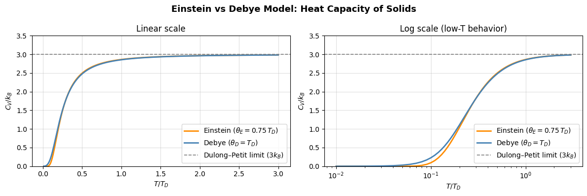

/tmp/ipykernel_2876/174881513.py:15: RuntimeWarning: overflow encountered in scalar power
  integrand = lambda x: (x**4 * np.exp(x)) / (np.exp(x) - 1)**2

Problems¶

Problem-1 1D energy profiles¶

Given an energy function $E(x)=Ax^4-Bx^2+C$ with constants $(A=1,B=4,C=1)$

Compute free energy difference between minima at temperature $kBT=1,10, 100$
Compute free energy around minima of size $\delta x = 0.1, 0.5, 1$

Problem-2 Maxwell-Boltzman¶

You are tasked with analyzing the behavior of non-interacting nitrogen gas molecules described by Maxwell-Boltzman distirbution:

f(v) = 4\pi \left( \frac{m}{2\pi k_B T} \right)^{3/2} v^2 e^{-\frac{mv^2}{2k_B T}}

(83)

Where:

$f(v)$ is the probability density for molecular speed $v$
$m$ is the mass of a nitrogen molecule
$k_B = 1.38 \times 10^{-23} \,\text{J/K}$ (Boltzmann constant)
$T$ is the temperature in Kelvin

Step 1: Plot the Maxwell-Boltzmann Speed Distribution

At room temperature (T = 300, 400, 500, 600 K), plot the distribution $f(v)$ for speeds ranging from 0 to 2000 m/s.

Step 2: Identify Most Probable, Average, and RMS Speeds

Compute and print:

The most probable speed $v_{mp} = \sqrt{\frac{2k_B T}{m}}$
The mean speed $\bar{v} = \sqrt{\frac{8k_B T}{\pi m}}$
The root mean square (RMS) speed $v_{rms} = \sqrt{\frac{3k_B T}{m}}$

Plot vertical lines on your plot from Step 1 to show these three characteristic speeds.

Step 3: Speed Threshold Analysis

Use numerical integration to calculate the fraction of molecules that have speeds:

(a) Greater than 1000 m/s
(b) Between 500 and 1000 m/s

Hint: Use scipy.integrate.quad to numerically integrate the Maxwell-Boltzmann distribution.

Problem-3 Elastic Collisions¶

Complete the lab

In this problem need to modify the code to add elastic collisions to the ideal gas simulations

Problem-4 Elementary derivation of Boltzmann’s distirbution¶

Let us do an elementary derivation of Boltzman distribution showing that when a macroscopic system is in equilibrium and coupled to a heat bath at temperatere $T$ we have a universal dependence of probability for finding system at different energies:

\boxed{P(r')/P(r)=e^{-\beta (U(r)-U(r'))}}

(84)

The essence of the derivation is this. Consider a vertical column of gas somehre in the mountains.

On one hand we have graviational force which acts on a column between $h, h+dh$ with cross section $A$ .
On the other hand we have pressure balance which thankfully keeps the molecules from dropping on the ground.
This means that we have a steady density of molecules at each distance $n(h)$ for a fixed $T$ . Write down this balance of forces (gravitational vs pressure ) and find show how density at $h$ , $n(h)$ is related to density at $h=0$ , $n(0)$ .

Tip: you may use $P=nkT$ for pressure and $mgh$ for the gravitational force)

Problem-5 2D diploes on a lattice¶

Consider a 2D square lattice with $M$ lattice points. On each point we have a mangeetic moment that can point in four possible directions: $+x, -x, +y, -y$ . Along $y$ axis, the dipole has the energy $\epsilon>0$ and along the x axis $\epsilon=0$ .

Dipoles are not interacting with each other and we also ingnore kinetic energy of diplos since they are fixed at lattice positions.

Write down parition function for this system $Z$
Compute the average energy.
Compute entropy per dipole $s(T)$ . Evaluate the difference $S(T=\infty)-S(T=0)$ ? Can you see a link with number of arrangements of dipols?
Compute microcanonical partition function $\Omega (N\epsilon)$
Show that we get the same entropy expression by using $NVE$ and $NVT$ ensembles.