Probability theory - Statmech4ChemBio

Probabilistic world of complex many particle systems¶

Characterizing many particle complex systems is best done via probabilistic approach.

Do you ever see most particles clumped in one corner?
Why does the gas spread out but never spontaneously un-spread?
What is the probability to find all of gas in on left side?
How does the probability of “all particles on the left half” scale with particle number N?
If you reverse animation would motion look natural?
What is the probability distribution of velocities of the gas particles?
If you take a snapshot, is “uniform density” guaranteed?
What does it mean for the system to be “in equilibrium” in this animation?

What is the probability of finding gas particle taking n out of N steps to the right?
How do we obtain probability distribution after N steps given probability for a single step?
Why is there tendency for probability distributions to evolve towards Gaussian?

Sample space¶

The sample space, often signified by an $\Omega$ is a set of all possible elementary events.
Elementary means the events can not be further broken down into simpler events. For instance, rolling a die can result in any one of six elementary events.
States of $\Omega$ are sampled during a system trial, which could be done via an experiment or simulation.

If our trial is a single roll of a six-sided die, then the sample has size $n(\Omega) = 6$

\Omega =\{1, 2, 3, 4, 5, 6 \}

(1)

A fair coin is tossed once has a sample size $n(\Omega) = 2$

\Omega = \{H, T \}

(2)

If a fair coin is tossed three times in a row, we will have sample space of size $n(\Omega) = 2^3$

\Omega = \{H,T\}^{3}= {HTT, THT, TTH, THH, HTH, HHT, HHH, TTT}

(3)

Position of an atom in a container of size $L_x$ along x. $n(\Omega)$ is a huge number. We will need some special tools to quantify.

\Omega = \{0... L_x\}

(4)

Events, micro and macro states¶

An event in probability theory refers to an outcome of an experiment. Event can contain one or more elementary events from $\Omega$ .
Event can be getting getting 5 on a die or getting any number less than 5.
In the context of statistical mechanics, we are going to call elementary events in $\Omega$ microstates and events containing multiple microstates as macrostates
- If we roll a single die there are six micostates. We can define a macrostate as an event $A$ of getting any number less than 4
$A= \{1, 2, 3 \}$
(5)
- Or we can create a macrostate $B$ containing only even numbers
$B = \{2, 4, 6 \}$
(6)
- IF we roll toss two coins microstates are HT, TH, HH, TT. We can define a macrostate $D$ of having 50% H and 50% T
$D = \{TH, HT\}$
(7)
- A microstate of a gas atom in 1D container could be its position x. A macrostate could be finding atom anywehere in the second half of the container
$C = \{L_x/2, ..., L_x \}$
(8)

Compute probabilities through counting¶

Visualizing events as Venn diagrams¶

# COllab has this but in local notebook you may want to install it
#!pip install matplotlib-venn #install if running locally
import matplotlib_venn as venn
import matplotlib.pyplot as plt

Omega = {1,2,3,4,5,6}

A = {1, 2, 3, 4, 5}

B = {4, 5, 6}

venn.venn2([A, B], set_labels=('A','B'))

print(len(A)/len(Omega))
print(len(B)/len(Omega))
print(len(A & B)/len(Omega))
print(len(A | B)/len(Omega))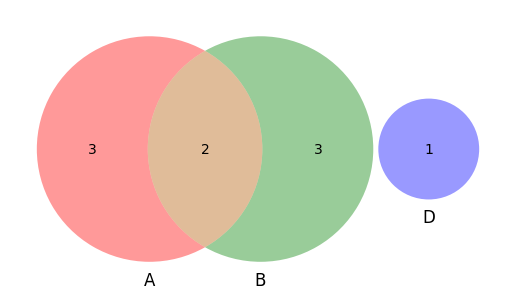

0.8333333333333334
0.5
0.3333333333333333
1.0

Probability Axioms¶

Bayes Theorem¶

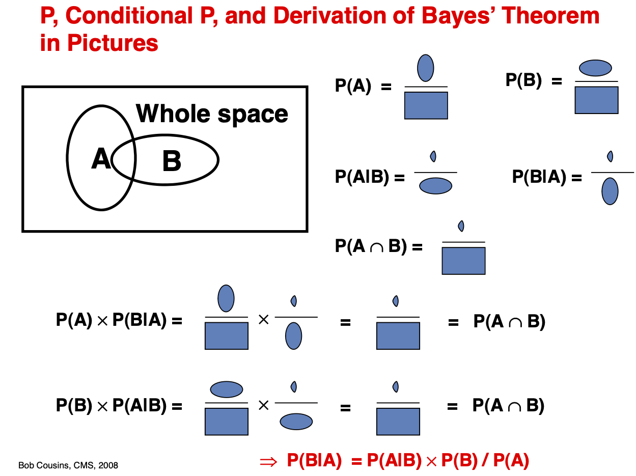
compton — **Joint Probability $P(A,B)$ :** Quantifies the probability of two or more events happening simultaneously. **Marginal Probability $P(A)$ :** Quantifies the probability of an event irrespective of the outcomes of other random variables. Is obtained by marginalization, summing over all possibilities of B. **Conditional Probability $P(A|B)$ :** Quantifies probability of event A given the information that event B happened.

Example of Using Bayes Formula to Test Hypothesis

A test for cancer is known to be 90% accurate either in detecting cancer if present or in giving an all-clear if cancer is absent.
The prevalence of cancer in the population is 1%. How worried should you be if you test positive? Try answering this question using Bayes’ theorem.

Prior, Posterior, and Likelihood

Bayes’ theorem provides a powerful framework for testing hypotheses or learning model parameters from data. While the mathematical formulation remains the same, the terminology used in Bayesian inference differs from the standard probability notation:

P(\theta | D) = \frac{P(D | \theta) \cdot P(\theta)}{P(D)}

(19)

where:

Prior: $P(\theta)$ represents our initial belief about the hypothesis or parameter before observing the data. For example, if we are tossing a coin, a reasonable prior might be a gaussian centered at $1/2$ or take unifrom distribution in absence of information.
Evidence: $P(D)$ is the probability of the observed data, also known as the marginal likelihood. It accounts for all possible parameter values and normalizes the posterior. For example, it is the probability of obtaining a specific sequence, such as $HTHH$ , given all possible biases of the coin.
Likelihood: $P(D | \theta)$ describes how probable the observed data is for a given parameter $\theta$ . E.g for sequence of $HTHH$ it will be $L(\theta)=\theta^3(1-\theta)$ giving probability of landing three H and 1 T.
Posterior: $P(\theta | D)$ is the updated probability of the hypothesis after incorporating the observed data. This is the key quantity in Bayesian inference, as it represents our revised belief about $\theta$ given the data. We can take value of $\theta$ corresponding to maximum of posterior to be most likely value of our parameter. For our case of uniform prior and likelhood the maxima will be $\theta = 3/4$ as we may expect.

Computing number of microstates via combinatorics¶

Binomial Distribution (Two-State Systems)

When molecules can be in two states (e.g., adsorbed vs. free, spin-up vs. spin-down), the number of ways to arrange $N$ molecules into state A $k$ and state B $N-k$ follows:

W(N, n) = \binom{N}{n} = \frac{N!}{N!(N-n)!}

(20)

For example, if $N$ gas molecules distribute between two parts of the box or spins occupying two energy levels, this formula gives the number of microstates for a given occupation $k$ .

Multinomial Distribution (Multiple States)

For systems with more than two states, such as molecules distributed among $m$ energy levels, the number of ways to assign $N$ molecules into states $n_1, n_2, ..., n_m$ with $\sum n_i = N$ is:

W(n_1, n_2, ..., n_m) = \frac{N!}{n_1! n_2! \cdots n_m!}.

(21)

Example: partitioning gas particles

Consider a container filled with 1000 atoms of Ar.

def gas_partition(k1=30, k2=30, k3=30):
    '''partitioning N gas molecules into regions k1, k2 and k3'''

    from scipy.special import factorial

    N = k1+k2+k3 

    return factorial(N) / (factorial(k1) * factorial(k2)* factorial(k3))

print( gas_partition(k1=50, k2=50, k3=0) )

print( gas_partition(k1=50, k2=49, k3=1) )

print( gas_partition(k1=50, k2=25, k3=25) )

print( gas_partition(k1=34, k2=33, k3=33) )

1.0089134454556417e+29
5.0445672272782094e+30
1.2753736048324953e+43
4.19244792425583e+45

Strinling approximation of factorial and binomials¶

import numpy as np
import matplotlib.pyplot as plt
import scipy.special as sp

# Define range for N
N_values = np.arange(1, 100, 1)

# Exact factorial using log(N!)
log_fact_exact = np.log(sp.factorial(N_values))

# Crude Stirling approximation
log_fact_crude = N_values * np.log(N_values) - N_values

# More accurate Stirling approximation
log_fact_accurate = N_values * np.log(N_values) - N_values + 0.5 * np.log(2 * np.pi * N_values)

# Plot comparisons
plt.figure(figsize=(10, 6))
plt.plot(N_values, log_fact_exact, label="Exact $log N!$", color="black", linewidth=2)
plt.plot(N_values, log_fact_crude, label="Crude Stirling Approximation", linestyle="--", color="red", linewidth=2)
plt.plot(N_values, log_fact_accurate, label="Accurate Stirling Approximation", linestyle=":", color="blue", linewidth=2)

plt.xlabel("N")
plt.ylabel("$\log N!$")
plt.title("Comparison of Stirling Approximations for $\log N!$")
plt.legend()
plt.grid(True)
plt.show()

<>:24: SyntaxWarning: invalid escape sequence '\l'
<>:25: SyntaxWarning: invalid escape sequence '\l'
<>:24: SyntaxWarning: invalid escape sequence '\l'
<>:25: SyntaxWarning: invalid escape sequence '\l'
/tmp/ipykernel_2745/2524245169.py:24: SyntaxWarning: invalid escape sequence '\l'
  plt.ylabel("$\log N!$")
/tmp/ipykernel_2745/2524245169.py:25: SyntaxWarning: invalid escape sequence '\l'
  plt.title("Comparison of Stirling Approximations for $\log N!$")

Problems¶

Problem 1: Counting Dies and coins¶

You flip a coin 10 times and record the data in the form of head/tails or 1s and 0s

What would be the probability of ladning 4 H’s?
What would be the probability of landing HHHTTTHHHT sequence?
In how many ways can we have 2 head and 8 tails in this experiments?
Okay, now you got tired of flipping coins and decide to play some dice. You throw die 10 times what is the probability of never landing number 6?
You throw a die 3 times what is the probability of obtaining a combined sum of 7?

Problem 2: Counting gas molecules¶

C^{N}_{k}

(32)

A container of volume $V$ contains $N$ molecules of a gas. We assume that the gas is dilute so that the position of any one molecule is independent of all other molecules. Although the density will be uniform on the average, there are fluctuations in the density. Divide the volume $V$ into two parts $V_1$ and $V_2$ , where $V = V_1 + V_2$ .

What is the probability p that a particular molecule is in each part?
What is the probability that $N_1$ molecules are in $V_1$ and $N_2$ molecules are in $V_2$ ?
What is the average number of molecules in each part?
What are the relative fluctuations of the number of particles in each part?

Project Porosity of materials¶

A simple model of a porous rock can be imagined by placing a series of overlap- ping spheres at random into a container of fixed volume $V$ . The spheres represent the rock and the space between the spheres represents the pores. If we write the volume of the sphere as v, it can be shown the fraction of the space between the spheres or the porosity $\phi$ is $\phi =e^{-Nv/V}$ , where $N$ is the number of spheres.

For simplicity, consider a 2D system, (e.g $v=\frac{1}{4}\pi d^2$ , see wiki if you forgot the formula). Write a python function which place disks of $d=1$ into a square box. The disks can overlap. Divide the box into square cells each of which has an edge length equal to the diameter of the disks. Find the probability of having 0, 1, 2, or 3 disks in a cell for $\phi$ = 0.03, 0.1, and 0.5.

You will need np.random.uniform() to randomly place N disks of volume v into volume V. Check out this cool python lib for porosity evaluation of materials R Shkarin, et al Plos Comp Bio 2019