Summary of Ensembles

The Big Picture: Why Multiple Ensembles?¶

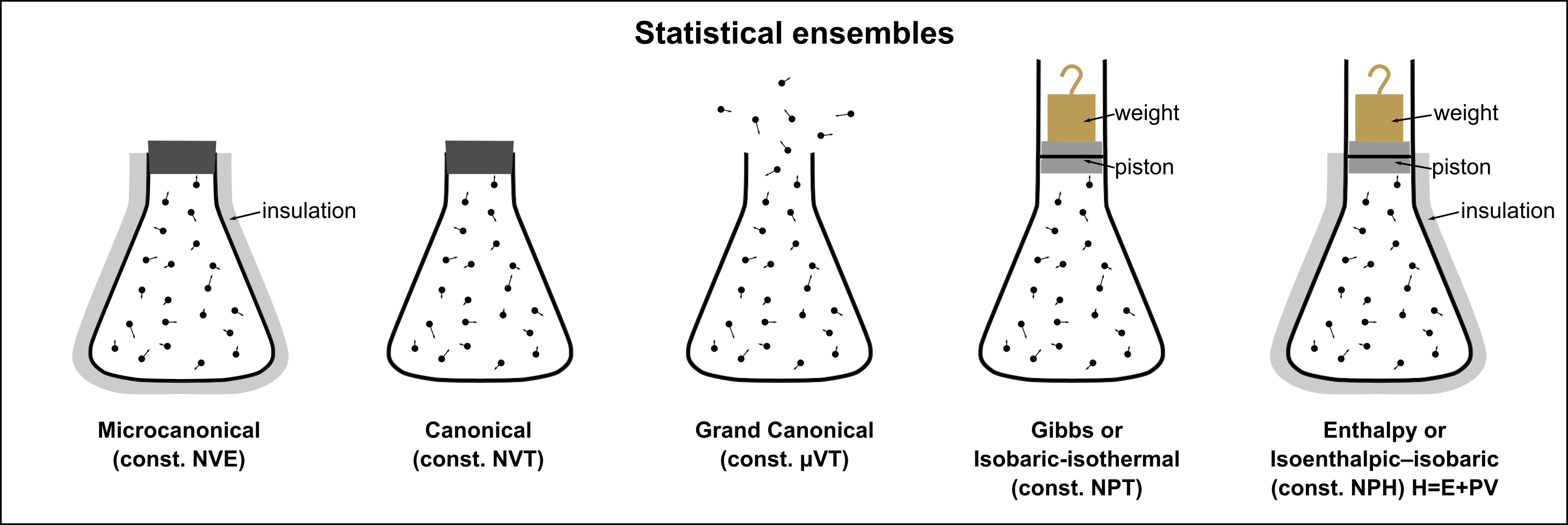
• All ensembles describe the same macroscopic physics in the thermodynamic limit. They differ only in which quantities are held fixed and which are allowed to fluctuate. The choice of ensemble is a choice of boundary conditions: what the system exchanges with its surroundings:

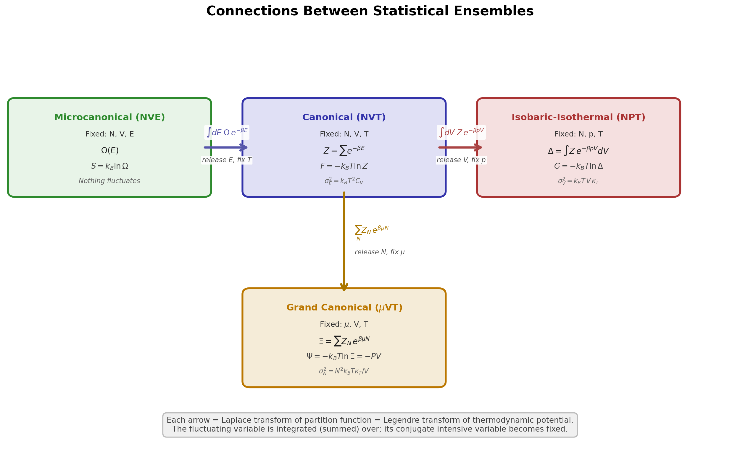
• Each arrow corresponds to placing the system in contact with a reservoir that controls the corresponding intensive variable ($T$, $p$, or $\mu$). Mathematically, each step is a Laplace transform of the partition function and a Legendre transform of the thermodynamic potential.

Entropy and the Origin of Ensemble Distributions¶

Entropy is given by the Shannon-Gibbs entropy formula:

where $p_i$ is the probability of the $i$th microstate.

Physical Constraints for Equilibrium¶

For a system to maintain equilibrium values, the microstate probabilities must satisfy the following conditions:

1. Normalization:

   $$\sum_{i} p_i = 1$$

   (4)

2. Constraint to Maintain the Expectation Value of an Observable $X$ (e.g., Energy or Volume):

   $$\sum_{i} p_i X_i = \langle X \rangle, \quad \sum_{i} p_i Y_i = \langle Y \rangle$$

   (5)

• The probability of a macrostate $(X, Y, \dots)$ follows the general form:

  $$P(X, Y, \dots) = \frac{e^{S(X, Y, \ldots)/k_B} \cdot e^{- \beta X} \cdot e^{- \gamma Y}\cdots}{Z}$$

  (6)
  $$Z(\beta, \gamma, \ldots) = \sum_{X, Y, \ldots} e^{S(X, Y, \ldots)/k_B}\, e^{- \beta X}\, e^{- \gamma Y}\cdots$$

  (7)

• Where $Z$ is a normalization factor called partition function

• Exponential dependence can also be understood as a consequence of exchange of (energy, volume, particles, etc.) with a large reservoir:

Comparison of Ensembles¶

• Entropy dependence $e^{S/k_B}$ is universal across all ensembles.

• Microstate probability follows different forms based on constraints from different thermodynamic potentials.

• Macrostate probability always includes an entropy term but is modified by energy, pressure, and chemical potential, depending on the ensemble.

Extensive vs Intensive Variables¶

• The total differential of internal energy $U$ in a thermodynamic system can be expressed in terms of its conjugate variables:

• where each pair $(X_i, f_i)$ represents a conjugate extensive and intensive variable respectively, such as:

  • $(S, T)$ — entropy and temperature,

  • $(V, -P)$ — volume and pressure,

  • $(N, \mu)$ — particle number and chemical potential,

  • $(M, B)$ — magnetization and magnetic field.

• Key principle: each ensemble is obtained by replacing one or more extensive natural variables of $U$ with the conjugate intensive variable. The reservoir fixes the intensive variable; the extensive variable fluctuates.

Laplace Transform and Ensemble Connections¶

• The Laplace transform connects different thermodynamic ensembles by integrating (summing) over a fluctuating extensive variable, weighted by the Boltzmann factor of the conjugate intensive variable. In the thermodynamic limit, the saddle-point approximation turns the Laplace transform into a Legendre transform.

• NVE $\to$ NVT (integrate over energy):

  $$Z(\beta, N, V) = \int dE \, \Omega(E)\, e^{-\beta E} \approx e^{\max_E [S(E)/k_B - \beta E]}$$

  (12)
  $$Z(\beta, N, V) = e^{-\beta [U - TS]} = e^{-\beta F(\beta, N, V)}$$

  (13)

• NVT $\to$ NPT (integrate over volume):

  $$\Delta(\beta, N, P) = \int dV \, Z(\beta, N, V)\, e^{-\beta P V} \approx e^{\max_V [-\beta F(V) - \beta P V]}$$

  (14)
  $$\Delta(\beta, N, P) = e^{-\beta [U - TS + PV]} = e^{-\beta G(\beta, N, P)}$$

  (15)

• NVT $\to$ $\mu$VT (sum over particle number):

  $$\Xi(\beta, \mu, V) = \sum_{N=0}^{\infty} Z(\beta, N, V)\, e^{\beta \mu N} \approx e^{\max_N [-\beta F(N) + \beta \mu N]}$$

  (16)
  $$\Xi(\beta, \mu, V) = e^{-\beta [U - TS - \mu N]} = e^{-\beta \Psi(\beta, \mu, V)} = e^{\beta PV}$$

  (17)

• Thus, free energy functions naturally emerge as Legendre transforms of internal energy through Laplace integration over fluctuating variables.

Legendre Transform and Thermodynamic Potentials¶

• The Legendre transformation allows us to reformulate equilibrium conditions (e.g., entropy maximization) in terms of more convenient variables (e.g., free energy minimization).

• This transformation makes it possible to work with temperature and pressure as control variables instead of entropy and volume.

• Free Energies as Legendre Transforms of Internal Energy:

Partition Functions and Legendre Transforms¶

• The partition function naturally follows the structure of a Legendre transform, as it is related to the thermodynamic potential via:

• The $\Psi$ is a thermodynamic potential obtained through Legendre transformation of the internal energy.

Fluctuation-Response Relations¶

• For a given extensive variable $X$ and its conjugate intensive variable $f$, the partition function $Z$ governs both the mean value and fluctuations of $X$.

• Mean value of $X$ at constant $f$:

  $$\langle X \rangle = \frac{\partial \log Z}{\partial (\beta f)}$$

  (20)

• Fluctuations of $X$ at constant $f$:

  $$\sigma^2_X = \langle X^2 \rangle - \langle X \rangle^2 = \frac{\partial^2 \log Z}{\partial (\beta f)^2}$$

  (21)

• This relation shows that fluctuations in $X$ are directly linked to the second derivative of the partition function, a fundamental result of statistical mechanics.

Energy fluctuations (Canonical Ensemble):¶

$$

$$

\sigma^2_E = k_B T^2 C_V

$$

$$

• where $C_V$ is the heat capacity at constant volume.

Volume fluctuations (Isothermal-Isobaric Ensemble):¶

$$

$$

\sigma^2_V = k_B T, V, \kappa_T

$$

$$

• where $\kappa_T = -\frac{1}{V}\left(\frac{\partial V}{\partial p}\right)_T$ is the isothermal compressibility.

Particle number fluctuations (Grand Canonical Ensemble):¶

$$

$$

\sigma^2_N = \frac{\langle N \rangle^2 k_B T \kappa_T}{V}

$$

$$

Unified pattern¶

Key Insights¶

• Relative fluctuations decrease as system size increases, typically scaling as $\sigma_X/\langle X \rangle \sim 1/\sqrt{N}$.

• Response functions (e.g., heat capacity, compressibility) determine fluctuation magnitude. Large response $\Leftrightarrow$ large fluctuations.

• Ensemble equivalence ensures that for large systems, different ensembles give equivalent macroscopic results, despite differing fluctuation magnitudes. This is precisely because relative fluctuations vanish as $N \to \infty$.

• Near phase transitions, response functions diverge ($C_V \to \infty$, $\kappa_T \to \infty$), and fluctuations become macroscopically large — this is when ensemble equivalence can break down.