Open Systems

Grand Canonical Ensemble¶

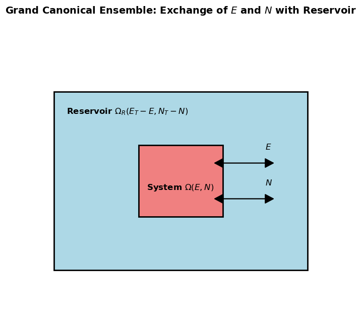
Consider small system $S$ in thermal and particle exchange with a large reservoir $R$ .
The total system $S + R$ is isolated: total energy $E_{\text{tot}} = E + E_R$ , total particle number $N_{\text{tot}} = N + N_R$ .
Total volume is constant, and the reservoir is much larger: $E \ll E_R$ , $N \ll N_R$ .

import matplotlib.pyplot as plt

# Create figure
fig, ax = plt.subplots(figsize=(7, 6))
ax.set_xlim(-1, 7)
ax.set_ylim(-1, 5)
ax.set_xticks([])
ax.set_yticks([])
ax.axis('off')

# Draw the large reservoir (outer rectangle)
reservoir = plt.Rectangle((0, 0), 6, 4, edgecolor='black', facecolor='lightblue', linewidth=2)
ax.add_patch(reservoir)

# Draw the small system (inner rectangle)
small_system = plt.Rectangle((2, 1.2), 2, 1.6, edgecolor='black', facecolor='lightcoral', linewidth=2)
ax.add_patch(small_system)

# Annotate the reservoir and system
ax.text(0.3, 3.5, r'Reservoir $\Omega_R(E_T - E, N_T - N)$', fontsize=12, color='black', fontweight='bold')
ax.text(2.2, 1.8, r'System $\Omega(E, N)$', fontsize=12, color='black', fontweight='bold')

# Draw arrows for energy exchange
ax.arrow(4, 2.4, 1, 0, head_width=0.2, head_length=0.2, fc='black', ec='black')
ax.arrow(5, 2.4, -1, 0, head_width=0.2, head_length=0.2, fc='black', ec='black')
ax.text(5, 2.7, r'$E$', fontsize=12, color='black', fontweight='bold')

# Draw arrows for particle exchange (offset vertically)
ax.arrow(4, 1.6, 1, 0, head_width=0.2, head_length=0.2, fc='black', ec='black')
ax.arrow(5, 1.6, -1, 0, head_width=0.2, head_length=0.2, fc='black', ec='black')
ax.text(5, 1.9, r'$N$', fontsize=12, color='black', fontweight='bold')

# Title
plt.suptitle(r'Grand Canonical Ensemble: Exchange of $E$ and $N$ with Reservoir', fontsize=14, fontweight='bold', y=1.05)

plt.tight_layout()
plt.show()

Grand Canonical Probability¶

The probability that the system has energy $E$ and particle number $N$ is proportional to the number of microstates of the reservoir with $E_R = E_{\text{tot}} - E$ , $N_R = N_{\text{tot}} - N$ :

P(E, N) \propto \Omega_R(E_{\text{tot}} - E, N_{\text{tot}} - N)

(1)

Define entropy of the reservoir $S_R = k_B \ln \Omega_R$ . Then:

\ln \Omega_R(E_R, N_R) = \ln \Omega_R(E_{\text{tot}} - E, N_{\text{tot}} - N)

(2)

Expand to first order:

\ln \Omega_R \approx \ln \Omega_R(E_{\text{tot}}, N_{\text{tot}}) - \left( \frac{\partial S_R}{\partial E_R} \right)_{N_R} \frac{E}{k_B} - \left( \frac{\partial S_R}{\partial N_R} \right)_{E_R} \frac{N}{k_B}

(3)

Use thermodynamic definitions:

\frac{1}{T} = \left( \frac{\partial S_R}{\partial E_R} \right)_{N_R}, \quad \frac{\mu}{T} = -\left( \frac{\partial S_R}{\partial N_R} \right)_{E_R}

(4)

\ln \Omega_R(E_R, N_R) = \text{const} - \frac{E}{k_B T} + \frac{\mu N}{k_B T}

(5)

P(E, N) \propto e^{-\beta (E - \mu N)}

(6)

Grand Canonical Distribution and Partition Function¶

Define the grand canonical partition function:

\Xi = \sum_N \sum_{\text{states at } N} e^{-\beta (E - \mu N)} = \sum_N z^N Z_N

(7)

where:

$z = e^{\beta \mu}$ is called the fugacity.
$Z_N = \sum_{\text{states at fixed } N} e^{-\beta E}$ is the canonical partition function at fixed $N$
The microstate probability in grand canonical ensemble is:

P_{\text{micro}}(E_i, N) = \frac{e^{-\beta (E_i - \mu N)}}{\Xi}

(8)

The macrostate probability over different energy values in grand canonical ensemble is:

P_{\text{macro}}(E, N) = \frac{\Omega(E) e^{-\beta (E - \mu N)}}{\Xi}

(9)

Connections with $NVE$ and $NVT$ ¶

Each ensemble arises from a different choice of what the system exchanges with its surroundings. The table below summarizes how the three ensembles we have encountered so far are related:

Property	$NVE$ (Microcanonical)	$NVT$ (Canonical)	$\mu VT$ (Grand Canonical)
Fixed variables	$N, V, E$	$N, V, T$	$\mu, V, T$
Fluctuating quantities	—	$E$	$E, N$
Exchange with reservoir	Nothing (isolated)	Energy	Energy + Particles
Partition function	$\Omega(E)$	$Z = \sum e^{-\beta E}$	$\Xi = \sum e^{-\beta(E - \mu N)}$
Thermodynamic potential	$S = k_B \ln \Omega$	$F = -k_BT \ln Z$	$\Psi = -k_BT \ln \Xi = -PV$
Fluctuation-response	—	$\sigma_E^2 = k_BT^2 C_V$	$\sigma_N^2 = \frac{N^2 k_BT \kappa_T}{V}$

Each successive ensemble is obtained by “opening up” one more variable: $NVE \xrightarrow{\text{allow } E \text{ to fluctuate}} NVT \xrightarrow{\text{allow } N \text{ to fluctuate}} \mu VT$ .
The corresponding partition function is a Laplace transform of the previous one, and the thermodynamic potential is related by a Legendre transform.

Statistical Dominance of Average Energy and Particle Number¶

Recall that the canonical ensemble emerges by weighting microcanonical contributions at different energies with an exponential factor $e^{-\beta E}$ .
Similarly, the grand canonical ensemble arises by further summing over all particle numbers $N$ , each weighted by the fugacity factor $e^{\beta \mu N}$ . This yields the grand canonical partition function:
$\Xi(T, V, \mu) = \sum_{N=0}^{\infty} \left[ \sum_i e^{-\beta E_i} \right] e^{\beta \mu N} = \sum_{N=0}^{\infty} Z(N, V, T) \, e^{\beta \mu N}$
(12)
In the thermodynamic limit, the sum is dominated by the most probable energy and particle number, giving:
$\Xi \approx e^{-\beta (F - \mu \bar{N})} = e^{-\beta (\bar{E} - T S - \mu \bar{N})} = e^{-\beta \Psi(T, V, \mu)}$
(13)
We identify a new thermodynamic potential for the grand canonical ensemble that plays same role as free energy in canonical ensemble:

:class: - Unknown Directive

$$
  \Psi(T, V, \mu) = E - T S - \mu N
$$

Thermodynamics and Legendre transform¶

In thermodynamics grand potential $\Psi$ is derived from the internal energy $E(S, V, N)$ via a Legendre transform that replaces the natural variables $S \to T$ and $N \to \mu$ :
$E(S, V, N) \rightarrow E - \left( \frac{\partial E}{\partial S} \right) S - \left( \frac{\partial E}{\partial N} \right) N = E - T S - \mu N$
(14)

Grand Potential and Pressure¶

Using Euler’s relation for extensive thermodynamic variables:
$E = T S + P V + \mu N$
(15)
Substituting into the definition of $\Psi$ , we find:
$\Psi = E - T S - \mu N = -P V$
(16)
Hence, the grand potential is directly related to the pressure and volume:
${\Psi(T, V, \mu) = -P V}$
(17)

Fluctuations in particle numbers¶

\langle N \rangle = \sum_i p_i N_i = \frac{\partial \log \Xi}{\partial (\beta \mu)}

(18)

\sigma_N^2 = \langle N^2 \rangle - \langle N \rangle^2 = \frac{\partial^2 \log \Xi}{\partial (\beta \mu)^2} = \frac{\partial \langle N \rangle}{\partial (\beta \mu)}

(19)

We once again find that the relative fluctuation of an extensive quantity scales as $N^{-1/2}$ , a consequence of extensivity and the law of large numbers:

\frac{\sigma_N}{\langle N \rangle} \sim O(N^{-1/2})

(20)

Using thermodynamics we could also link number fluctuations with isothermal compressibility $\kappa_T$

\kappa_T = -\frac{1}{V} \frac{\partial V}{\partial p} \geq 0

(21)

The relationship is analogous to what we had established in $NVT$ between energy fluctuations and heat capacity.

\sigma_N^2 = \frac{N^2 k_B T \kappa_T}{V} \sim O(N)

(22)

It takes a bit more work manipulating variables to get there in this case. See below for derivation:

Number fluctuations and isothermal compressibility

Let $N = \langle N \rangle$ (average particle number) and $n = \frac{N}{V}$ (number density)
Define isothermal compressibility:
$\kappa_T = -\frac{1}{V} \left( \frac{\partial V}{\partial p} \right)_{T,N}$
(23)
We’ll now recast this in terms of quantities more natural in the grand canonical ensemble — like $\mu$ and $N$ .
We start from grand canonical potential:

\Psi(T, V, \mu) = -pV

(24)

Take the total differential:

d\Psi = -S\,dT - p\,dV - N\,d\mu

(25)

\left( \frac{\partial \Psi}{\partial \mu} \right)_{T,V} = -N \quad \Rightarrow \quad \left( \frac{\partial (-pV)}{\partial \mu} \right)_{T,V} = -N

(26)

-V \left( \frac{\partial p}{\partial \mu} \right)_{T,V} = -N \quad \Rightarrow \quad \left( \frac{\partial p}{\partial \mu} \right)_T = \frac{N}{V} = n

(27)

\boxed{ n = \left( \frac{\partial p}{\partial \mu} \right)_T }

(28)

This identity is valid generally in the grand canonical ensemble and is a key link between statistical mechanics and thermodynamics.
This tells us: if you increase the chemical potential, the pressure increases, and so does particle density.
Now we differentiate again:

\left( \frac{\partial n}{\partial \mu} \right)_T = \left( \frac{\partial^2 p}{\partial \mu^2} \right)_T

(29)

That’s great, but we still want to connect this to compressibility, which involves how volume or density responds to pressure.
From chain rule we get

\left( \frac{\partial n}{\partial \mu} \right)_T = \left( \frac{\partial n}{\partial p} \right)_T \left( \frac{\partial p}{\partial \mu} \right)_T = \left( \frac{\partial n}{\partial p} \right)_T \cdot n

(30)

Now recall:

\kappa_T = \frac{1}{n} \left( \frac{\partial n}{\partial p} \right)_T \quad \Rightarrow \quad \left( \frac{\partial n}{\partial p} \right)_T = n \kappa_T

(31)

\left( \frac{\partial n}{\partial \mu} \right)_T = n \cdot (n \kappa_T) = n^2 \kappa_T

(32)

\left( \frac{\partial N}{\partial \mu} \right)_{T,V} = V \left( \frac{\partial n}{\partial \mu} \right) = V n^2 \kappa_T = \frac{N^2 \kappa_T}{V}

(33)

\boxed{ \left( \frac{\partial \langle N \rangle}{\partial \mu} \right)_{T,V} = \frac{N^2 \kappa_T}{V} }

(34)

And plugging into the fluctuation formula:

\sigma_N^2 = k_B T \cdot \left( \frac{\partial \langle N \rangle}{\partial \mu} \right) = \frac{N^2 k_B T \kappa_T}{V}

(35)

Intuition for Chemical Potential¶

In the canonical ensemble, temperature controls energy flow: energy flows from hot to cold until temperatures equalize. Chemical potential plays the exact same role for particle flow: particles flow from regions of high $\mu$ to regions of low $\mu$ until chemical potentials equalize across the system.
For an ideal gas, $\mu = k_BT \ln(n\lambda^3)$ , which reveals two competing effects:
- $\mu$ increases with density $n$ : a crowded system has high chemical potential and tends to “push” particles out
- $\mu$ decreases with temperature $T$ (through $\lambda \propto T^{-1/2}$ ): thermal agitation makes adding a particle less costly in free energy
In the classical regime ( $n\lambda^3 \ll 1$ ), the chemical potential is always negative. This means adding a particle to a dilute gas at fixed $T$ and $V$ always lowers the free energy: the entropy gain from having more accessible states outweighs the (zero) interaction energy cost.
The chemical potential becomes zero and eventually positive only in the quantum regime ( $n\lambda^3 \gtrsim 1$ ), where quantum statistics (Fermi-Dirac or Bose-Einstein) become important.

import numpy as np
import matplotlib.pyplot as plt

n_lambda3 = np.linspace(0.001, 0.8, 500)  # classical regime n*lambda^3 << 1
mu_over_kT = np.log(n_lambda3)

fig, ax = plt.subplots(figsize=(7, 4))
ax.plot(n_lambda3, mu_over_kT, lw=2, color='steelblue')
ax.axhline(0, color='gray', ls='--', lw=1)
ax.fill_between(n_lambda3, mu_over_kT, 0, where=(n_lambda3 < 0.3), alpha=0.15, color='steelblue')
ax.set_xlabel(r'$n\lambda^3$ (dimensionless density)', fontsize=12)
ax.set_ylabel(r'$\mu / k_BT$', fontsize=12)
ax.set_title('Chemical Potential of Classical Ideal Gas', fontsize=14, weight='bold')
ax.annotate('Classical regime\n' + r'($n\lambda^3 \ll 1$, $\mu < 0$)',
            xy=(0.1, np.log(0.1)), fontsize=11,
            xytext=(0.4, -4), arrowprops=dict(arrowstyle='->', color='red', lw=1.5))
ax.annotate(r'$\mu = 0$ at $n\lambda^3 = 1$' + '\n(quantum degeneracy)',
            xy=(0.75, np.log(0.75)), fontsize=10,
            xytext=(0.4, -1), arrowprops=dict(arrowstyle='->', color='darkgreen', lw=1.5))
ax.grid(True, alpha=0.3)
ax.set_xlim(0, 0.8)
ax.set_ylim(-7, 0.5)
plt.tight_layout()
plt.show()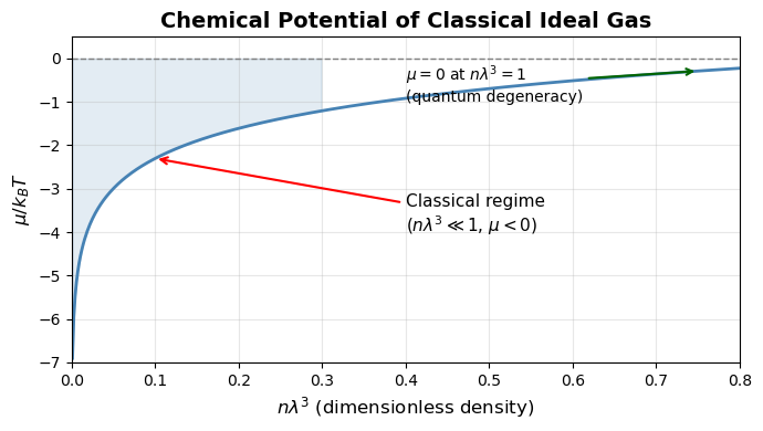

Ideal Gas in the Grand Canonical Ensemble¶

We begin by considering an ideal gas of indistinguishable, non-interacting particles in a volume $V$ , in thermal and chemical equilibrium with a reservoir at temperature $T$ and chemical potential $\mu$ .
The canonical partition function for $N$ particles is:

Z(T, V, N) = \frac{1}{N!} \left( \frac{V}{\lambda^3} \right)^N

(36)

Where the thermal de Broglie wavelength is:

\lambda = \frac{h}{\sqrt{2 \pi m k_B T}}

(37)

Grand Canonical Partition Function¶

To account for fluctuations in particle number, we compute the grand canonical partition function:

\Xi(T, V, \mu) = \sum_{N=0}^\infty Z(T, V, N)\, e^{\beta \mu N} = \sum_{N=0}^\infty \frac{1}{N!} \left( e^{\beta \mu} \frac{V}{\lambda^3} \right)^N = \exp\left( z \frac{V}{\lambda^3} \right)

(38)

Fugacity: $z = e^{\beta \mu}$ , a dimensionless measure of how favorable it is to add a particle to the system.
The average particle number is then obtained by taking first derivative with respect to $\mu$

\langle N \rangle = \frac{\partial \log \Xi}{\partial (\beta \mu)} = \frac{V}{\lambda^3} e^{\beta \mu} = z \frac{V}{\lambda^3}

(39)

Chemical Potential in Terms of Pressure and Density¶

We can invert the relation for $\langle N \rangle$ to express the chemical potential:

\mu = k_B T \log \left( \frac{N \lambda^3}{V} \right)

(40)

Noting that for an ideal gas $p = \frac{N k_B T}{V}$ , this becomes:

Number Fluctuations¶

In the grand canonical ensemble, number fluctuations are given by:

\sigma_N^2 = \langle N^2 \rangle - \langle N \rangle^2 = \frac{\partial \langle N \rangle}{\partial (\beta \mu)} = \langle N \rangle = N

(42)

So the standard deviation $\sigma_N \sim \sqrt{N}$ , and relative fluctuations vanish as $N^{-1/2}$ in the thermodynamic limit.

Isothermal Compressibility¶

We relate number fluctuations to the isothermal compressibility $\kappa_T$ :

\sigma_N^2 = \frac{N^2 k_B T \kappa_T}{V} \quad \Rightarrow \quad \kappa_T = \frac{V}{N^2 k_B T} \cdot \sigma_N^2 = \frac{V}{N k_B T} = \frac{1}{p}

(43)

This is the well-known result for the ideal gas compressibility:
$\kappa_T = \frac{1}{p} \geq 0$ , a positive quantity ensuring mechanical stability.

Molecular Adsorption of Ideal Gas on Surfaces¶

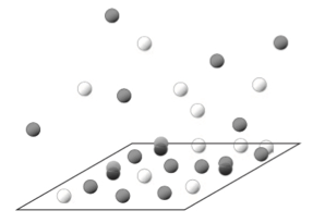
One Site–One Molecule Model¶

We consider a simple model where each adsorption site can hold at most one molecule. The surface is in thermal and chemical equilibrium with a gas reservoir at temperature $T$ and chemical potential $\mu$ .

Each site has two possible states:
- Empty: energy $E = 0$
- Occupied: energy $E = \epsilon$
Then the grand partition function for a single site is:

\Xi = 1 + e^{-\beta(\epsilon - \mu)}

(44)

$N$ Independent Sites¶

If there are $N$ independent and identical adsorption sites, then the total grand partition function is:

\Xi_{\text{total}} = \Xi^N = \left(1 + e^{-\beta(\epsilon - \mu)}\right)^N

(45)

Since the sites do not interact, their contributions multiply.

Average Number of Adsorbed Molecules¶

The average occupation number per site is:

\langle n \rangle = \frac{1}{e^{-\beta(\mu - \epsilon)} + 1}

(46)

The total number of adsorbed molecules is:

\langle N_{\text{ads}} \rangle = N \langle n \rangle = \frac{N}{e^{-\beta(\mu - \epsilon)} + 1}

(47)

Average Energy¶

The average energy per site is:

\langle E \rangle = \epsilon \langle n \rangle

(48)

The total energy of the system is:

\langle E_{\text{total}} \rangle = N \epsilon \langle n \rangle

(49)

Connecting to Pressure¶

For an ideal gas in the reservoir, the chemical potential is related to pressure via:

\mu = k_B T \log \left( \frac{p}{p_0} \right)

(50)

where $p_0$ is a reference pressure determined by the internal partition function of the gas.

Substituting this into the expression for $\langle n \rangle$ :

\langle n \rangle = \frac{p}{p_0 e^{\beta \epsilon} + p}

(51)

and thus the total number of adsorbed molecules becomes:

\langle N_{\text{ads}} \rangle = N \cdot \frac{p}{p_0 e^{\beta \epsilon} + p}

(52)

This is the Langmuir adsorption isotherm, describing how the fraction of occupied adsorption sites depends on gas pressure. It captures saturation behavior as $p \to \infty$ , where $\langle n \rangle \to 1$ .

import matplotlib.pyplot as plt
import numpy as np

# Use dimensionless units: energies in units of epsilon
epsilon = 1.0  # binding energy (reference unit)
p0 = 1.0       # reference pressure

p = np.linspace(0, 10, 500)

fig, ax = plt.subplots(figsize=(8, 5))
for kT in [0.2, 0.5, 1.0, 2.0, 5.0]:
    n_avg = p / (p0 * np.exp(epsilon / kT) + p)
    ax.plot(p, n_avg, lw=2, label=rf'$k_BT/\epsilon = {kT}$')

ax.set_xlabel(r'Pressure $p / p_0$', fontsize=12)
ax.set_ylabel(r'Average Occupancy $\langle n \rangle$', fontsize=12)
ax.set_title('Langmuir Adsorption Isotherm', fontsize=14, weight='bold')
ax.legend(fontsize=11)
ax.set_ylim(0, 1.05)
ax.set_xlim(0, 10)
ax.axhline(1.0, color='gray', ls='--', lw=1, alpha=0.5)
ax.grid(True, alpha=0.3)
plt.tight_layout()
plt.show()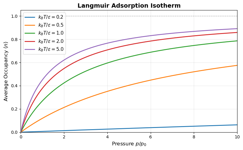

Chemical Equilibrium in gas mixtures¶

For each species $i$ , the canonical partition function is:

Z_i = \frac{z_i^{N_i}}{N_i!} \quad \text{with} \quad z_i = \frac{V}{\lambda_i^3} q_i^{\text{int}}(T)

(53)

where:

$\lambda_i = \frac{h}{\sqrt{2\pi m_i k_B T}}$ is the thermal wavelength,
$q_i^{\text{int}}$ is the internal partition function (rotations, vibrations, etc.),
$N_i$ is the number of molecules of species $i$ .
For convenience lets use the Helmholtz free energy (same result with Gibbs Free energy):

F = -k_B T \log Z = -k_B T \sum_i \log Z_i = -k_B T \sum_i \left[ N_i \log z_i - \log N_i! \right]

(54)

Using Stirling’s approximation $\log N_i! \approx N_i \log N_i - N_i$ :

F \approx k_B T \sum_i N_i \left( \log \frac{N_i}{z_i} - 1 \right)

(55)

Equilibrium via minimization of free energy¶

Now, we consider a chemical reaction:

aA + bB \rightleftharpoons cC + dD

(56)

We introduce an extent of reaction $\xi$ which measures how far reaction has progressed from reactants to products:

N_A = N_A^0 - a\xi,\quad N_B = N_B^0 - b\xi,\quad N_C = N_C^0 + c\xi,\quad N_D = N_D^0 + d\xi

(57)

We minimize $F(\xi)$ at constant $T, V$ by setting:

\frac{dF}{d\xi} = 0

(58)

Computing the derivative:

\frac{dF}{d\xi} = \sum_i \frac{\partial F}{\partial N_i} \frac{dN_i}{d\xi} = \sum_i \mu_i \nu_i = 0

(59)

with $\nu_i$ the stoichiometric coefficient ( $< 0$ for reactants, $> 0$ for products). Or we can write it in terms of positive stoichiometric coefficients:

\mu_i = \frac{\partial F}{\partial N_i} = k_B T \log \left( \frac{N_i}{z_i} \right)

(61)

So the equilibrium condition is:

\sum_i \nu_i \mu_i = k_B T \sum_i \nu_i \log \left( \frac{N_i}{z_i} \right) = 0

(62)

Exponentiating both sides we relate ratio of equilibrium numbers or concentrations to partition functions

\prod_i \left( \frac{N_i}{z_i} \right)^{\nu_i} = 1

(63)

Example: Chemical Equilibrium

Simple example using the reaction of $H_2+I_2$

\text{H}_2 + \text{I}_2 \rightleftharpoons 2\text{HI}

(65)

Step 1: Write equilibrium constant in terms of partition functions

K = \frac{(z_{\text{HI}}/V)^2}{(z_{\text{H}_2}/V)(z_{\text{I}_2}/V)} = \frac{z_{\text{HI}}^2}{z_{\text{H}_2} z_{\text{I}_2}}

(66)

Notice that all volume terms coming from translational part of partition function cancel out!

K(T) = \frac{q_{\text{HI}}^2}{q_{\text{H}_2} q_{\text{I}_2}} \quad \text{where} \quad q_i = \frac{z_i}{V}

(67)

Each $z_i = \frac{V}{\lambda_i^3} q_i^{\text{int}}(T)$ , so $q_i = \frac{q_i^{\text{int}}(T)}{\lambda_i^3}$ .

Step 2: Plug into expression for $K$

K(T) = \frac{\left( \frac{q_{\text{HI}}^{\text{int}}}{\lambda_{\text{HI}}^3} \right)^2} {\left( \frac{q_{\text{H}_2}^{\text{int}}}{\lambda_{\text{H}_2}^3} \right) \left( \frac{q_{\text{I}_2}^{\text{int}}}{\lambda_{\text{I}_2}^3} \right)}

(68)

This gives $K$ in terms of molecular properties at temperature $T$ . No volume dependence remains.

Grand Canonical Monte Carlo: Particle Number Fluctuations in Action¶

The formulas above predict that particle number fluctuates in the grand canonical ensemble with $\sigma_N \sim \sqrt{N}$ . We can see this directly using a simple Grand Canonical Monte Carlo (GCMC) simulation on a lattice. At each step, we randomly attempt to insert or delete a particle, accepting moves with probability determined by $\beta\mu$ .

How the GCMC algorithm works

We are going to learn how to simulate lattice systems using Monte-Carlo algorithm in subsequent sections. But we the idea is simple enough that we can state it here. At each step we do three things:

Pick a random site on the lattice.
If the site is empty, attempt to insert a particle:
- Compute the energy change $\Delta E$ from adding the particle
- Accept with probability $\min\left(1,\; e^{-\beta(\Delta E - \mu)}\right)$
If the site is occupied, attempt to delete the particle:
- Compute the energy change $\Delta E$ from removing it
- Accept with probability $\min\left(1,\; e^{-\beta(\Delta E + \mu)}\right)$

For a non-interacting lattice gas ( $\Delta E = 0$ ), the acceptance simplifies to:

Insert: $\min(1, e^{\beta\mu})$
Delete: $\min(1, e^{-\beta\mu})$

Why it works: After many steps, the system samples the correct equilibrium distribution of $N$ , and we can directly measure $\langle N \rangle$ , $\sigma_N$ , and any other observable. The reason is that we engineered acceptance rule to satisfy the so called detailed balance with respect to the grand canonical distribution $P \propto e^{-\beta(E - \mu N)}$ .

Intuition for $\mu$ :

$\beta\mu \ll 0$ : insertions are rarely accepted, deletions are easy $\Rightarrow$ low density
$\beta\mu = 0$ : insertions and deletions equally likely $\Rightarrow$ half-filled
$\beta\mu \gg 0$ : insertions are easy, deletions are rarely accepted $\Rightarrow$ high density

import numpy as np
import matplotlib.pyplot as plt
from matplotlib import animation
from matplotlib.colors import ListedColormap
from IPython.display import HTML

def gcmc_animation_frames(beta_mu, L=25, n_steps=30000, n_frames=80):
    """Run GCMC and collect frames for animation."""
    grid = np.zeros((L, L), dtype=int)
    N = 0
    p_ins = min(1.0, np.exp(beta_mu))
    p_del = min(1.0, np.exp(-beta_mu))
    
    steps_per_frame = n_steps // n_frames
    frames = []
    N_vals = []
    
    for step in range(n_steps):
        x, y = np.random.randint(0, L, 2)
        if grid[x, y] == 0:
            if np.random.rand() < p_ins:
                grid[x, y] = 1; N += 1
        else:
            if np.random.rand() < p_del:
                grid[x, y] = 0; N -= 1
        if (step + 1) % steps_per_frame == 0:
            frames.append(grid.copy())
            N_vals.append(N)
    return frames, N_vals

# Generate frames for low and high mu
np.random.seed(42)
frames_low, N_low = gcmc_animation_frames(-2, L=25, n_steps=30000, n_frames=80)
frames_high, N_high = gcmc_animation_frames(2, L=25, n_steps=30000, n_frames=80)

cmap = ListedColormap(['#f0f0f0', '#2c7bb6'])

fig, (ax1, ax2) = plt.subplots(1, 2, figsize=(10, 4.5))
im1 = ax1.imshow(frames_low[0], cmap=cmap, vmin=0, vmax=1, interpolation='nearest')
im2 = ax2.imshow(frames_high[0], cmap=cmap, vmin=0, vmax=1, interpolation='nearest')

ax1.set_title(r'Low $\mu$: $\beta\mu = -2$', fontsize=13, fontweight='bold')
ax2.set_title(r'High $\mu$: $\beta\mu = +2$', fontsize=13, fontweight='bold')

for ax in [ax1, ax2]:
    ax.set_xticks([]); ax.set_yticks([])
    for spine in ax.spines.values():
        spine.set_linewidth(2)

txt1 = ax1.text(0.5, -0.07, '', transform=ax1.transAxes, ha='center', fontsize=11)
txt2 = ax2.text(0.5, -0.07, '', transform=ax2.transAxes, ha='center', fontsize=11)

fig.suptitle('GCMC Animation: Lattice Filling at Different Chemical Potentials',
             fontsize=14, fontweight='bold')
plt.tight_layout()

def update(frame):
    im1.set_data(frames_low[frame])
    im2.set_data(frames_high[frame])
    L = 25
    txt1.set_text(rf'$N = {N_low[frame]}$, $\theta = {N_low[frame]/(L*L):.2f}$')
    txt2.set_text(rf'$N = {N_high[frame]}$, $\theta = {N_high[frame]/(L*L):.2f}$')
    return [im1, im2, txt1, txt2]

plt.close(fig)
ani = animation.FuncAnimation(fig, update, frames=len(frames_low), 
                               interval=80, blit=True)
HTML(ani.to_jshtml())

Loading...

import numpy as np
import matplotlib.pyplot as plt

def gcmc_lattice_gas(beta_mu, n_steps=50000, L=20):
    """Simple GCMC for non-interacting lattice gas.
    Each lattice site is either empty (0) or occupied (1).
    Acceptance probability for insertion/deletion depends on beta*mu.
    """
    grid = np.zeros((L, L), dtype=int)
    N = 0
    N_history = []
    p_accept_insert = min(1.0, np.exp(beta_mu))
    p_accept_delete = min(1.0, np.exp(-beta_mu))
    
    for _ in range(n_steps):
        x, y = np.random.randint(0, L, 2)
        if grid[x, y] == 0:  # try to insert
            if np.random.rand() < p_accept_insert:
                grid[x, y] = 1
                N += 1
        else:  # try to delete
            if np.random.rand() < p_accept_delete:
                grid[x, y] = 0
                N -= 1
        N_history.append(N)
    return np.array(N_history)

# Run GCMC at different chemical potentials
fig, axes = plt.subplots(1, 2, figsize=(13, 4.5))
colors = ['#1f77b4', '#ff7f0e', '#2ca02c']
beta_mu_values = [-2, 0, 1.5]

for beta_mu, color in zip(beta_mu_values, colors):
    N_hist = gcmc_lattice_gas(beta_mu, n_steps=50000)
    burn_in = 5000
    N_eq = N_hist[burn_in:]
    
    # Time series (last 10000 steps)
    axes[0].plot(N_hist[-10000:], alpha=0.7, color=color, 
                 label=rf'$\beta\mu = {beta_mu}$')
    
    # Histogram
    rel_fluct = np.std(N_eq) / np.mean(N_eq) if np.mean(N_eq) > 0 else 0
    axes[1].hist(N_eq, bins=30, alpha=0.5, density=True, color=color,
                 label=rf'$\beta\mu={beta_mu}$, $\sigma_N/\langle N\rangle={rel_fluct:.3f}$')

axes[0].set_xlabel('MC Step', fontsize=12)
axes[0].set_ylabel('N (particle number)', fontsize=12)
axes[0].set_title('Particle Number Fluctuations (GCMC)', fontsize=13, weight='bold')
axes[0].legend(fontsize=10)
axes[0].grid(True, alpha=0.3)

axes[1].set_xlabel('N', fontsize=12)
axes[1].set_ylabel('P(N)', fontsize=12)
axes[1].set_title('Distribution of Particle Number', fontsize=13, weight='bold')
axes[1].legend(fontsize=9)
axes[1].grid(True, alpha=0.3)

plt.tight_layout()
plt.show()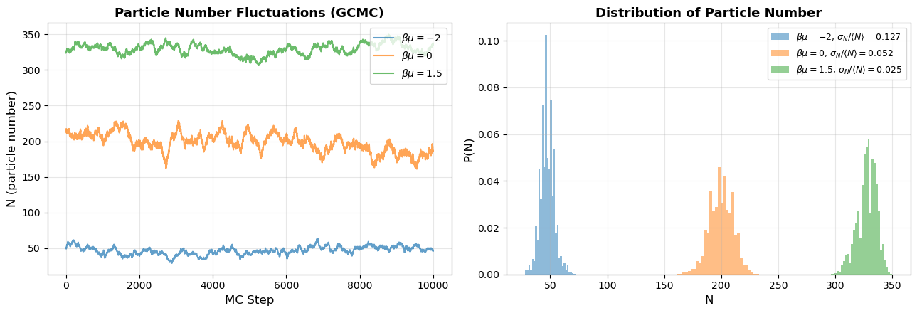

Isothermal-Isobaric (NPT) Ensemble¶

Most experiments in chemistry and biology are performed at constant temperature and pressure (e.g., reactions in open flasks, protein folding in solution). The appropriate statistical ensemble is the NPT ensemble, where the system exchanges energy and volume with a reservoir while keeping particle number fixed.

Derivation¶

Consider a system $S$ in thermal and mechanical contact with a large reservoir $R$ . The total system is isolated with fixed total energy $E_{\text{tot}} = E + E_R$ and total volume $V_{\text{tot}} = V + V_R$ .
The probability of finding the system in a state with energy $E$ and volume $V$ is:

P(E, V) \propto \Omega_R(E_{\text{tot}} - E,\, V_{\text{tot}} - V)

(69)

Expanding the reservoir entropy to first order (same logic as for NVT and $\mu$ VT):

\ln \Omega_R \approx \text{const} - \frac{E}{k_BT} - \frac{pV}{k_BT}

(70)

where we used:

\frac{1}{T} = \left(\frac{\partial S_R}{\partial E_R}\right)_{V_R}, \qquad \frac{p}{T} = \left(\frac{\partial S_R}{\partial V_R}\right)_{E_R}

(71)

This gives the NPT probability distribution:

P(E, V) \propto e^{-\beta(E + pV)}

(72)

Partition Function and Gibbs Free Energy¶

The thermodynamic potential is the Gibbs free energy:

G(T, p, N) = -k_BT \ln \Delta = E - TS + pV = H - TS

(74)

where $H = E + pV$ is the enthalpy.

The Gibbs free energy arises from the internal energy via Legendre transform replacing $S \to T$ and $V \to p$ :

E(S, V, N) \rightarrow E - TS + pV = G(T, p, N)

(75)

Volume Fluctuations¶

Just as energy fluctuates in NVT and particle number fluctuates in $\mu$ VT, volume fluctuates in NPT:

\langle V \rangle = -\frac{\partial \ln \Delta}{\partial (\beta p)}

(76)

\sigma_V^2 = \langle V^2 \rangle - \langle V \rangle^2 = -\frac{\partial \langle V \rangle}{\partial (\beta p)} = k_BT V \kappa_T

(77)

The relative volume fluctuation follows the same $N^{-1/2}$ scaling:

\frac{\sigma_V}{\langle V \rangle} = \sqrt{\frac{k_BT \kappa_T}{V}} \sim O(N^{-1/2})

(78)

Complete Ensemble Comparison¶

Property	$NVE$	$NVT$	$NPT$	$\mu VT$
Fixed	$N, V, E$	$N, V, T$	$N, p, T$	$\mu, V, T$
Fluctuating	—	$E$	$E, V$	$E, N$
Partition fn	$\Omega$	$Z$	$\Delta$	$\Xi$
Potential	$S$	$F = E - TS$	$G = E - TS + pV$	$\Psi = E - TS - \mu N$
Fluctuation-response	—	$\sigma_E^2 = k_BT^2 C_V$	$\sigma_V^2 = k_BT V \kappa_T$	$\sigma_N^2 = \frac{N^2 k_BT \kappa_T}{V}$

Problems¶

$NVT-NVE-\mu V T$ ¶

Consider a three level single particle system with five microstates with energies 0, ε, ε, ε, and 2ε. What is $\Omega(\epsilon, n)$ n=0,1,2 for this system? What is the mean energy of the system if it is in equilibrium with a heat bath at temperature T ?
Derive an expression for the chemical potential of an ideal gas using classical mechanics model for energy $E=\frac{p^2}{2m}$ in the $\mu VT$ ensemble evaluate the fluctuations in particle number.
Consider a system in equilibrium with a heat bath at temperature $T$ and a particle reservoir at chemical potential $\mu$ . The system can have a minimum of one and a maximum of four distinguishable particles. The particles in the system do not interact and can be in one of two states with energies zero or $\Delta$ . Determine the (grand) partition function of the system.
Combine the Gibbs formula of Entropy $S=-k_B \sum_i p_i log p_i$ with the Grand canonical probability distribution $P(E_i,N)=\frac{e^{-\beta E_i+ \beta \mu N}}{\Xi}$ to show that $\beta PV=\log \Xi$
Derive partition function for a pressure ensemble $(T, p, N)$ and show its connection with microcanonical ensemble $N V E$
At a given temperature T a surface with $N_0$ adsorption centers has on average $N\neq N_0$ number of adsorbed molecules. Suppose that there are no interactions between molecules.
- Show that the chemical potential of adsorbed gas is given by: $\mu = k_B T log \frac{N}{N_0 - N a(T)}$
- What is the meaning of $a(T)$