Simulation of Cu atoms
 {width=30%}
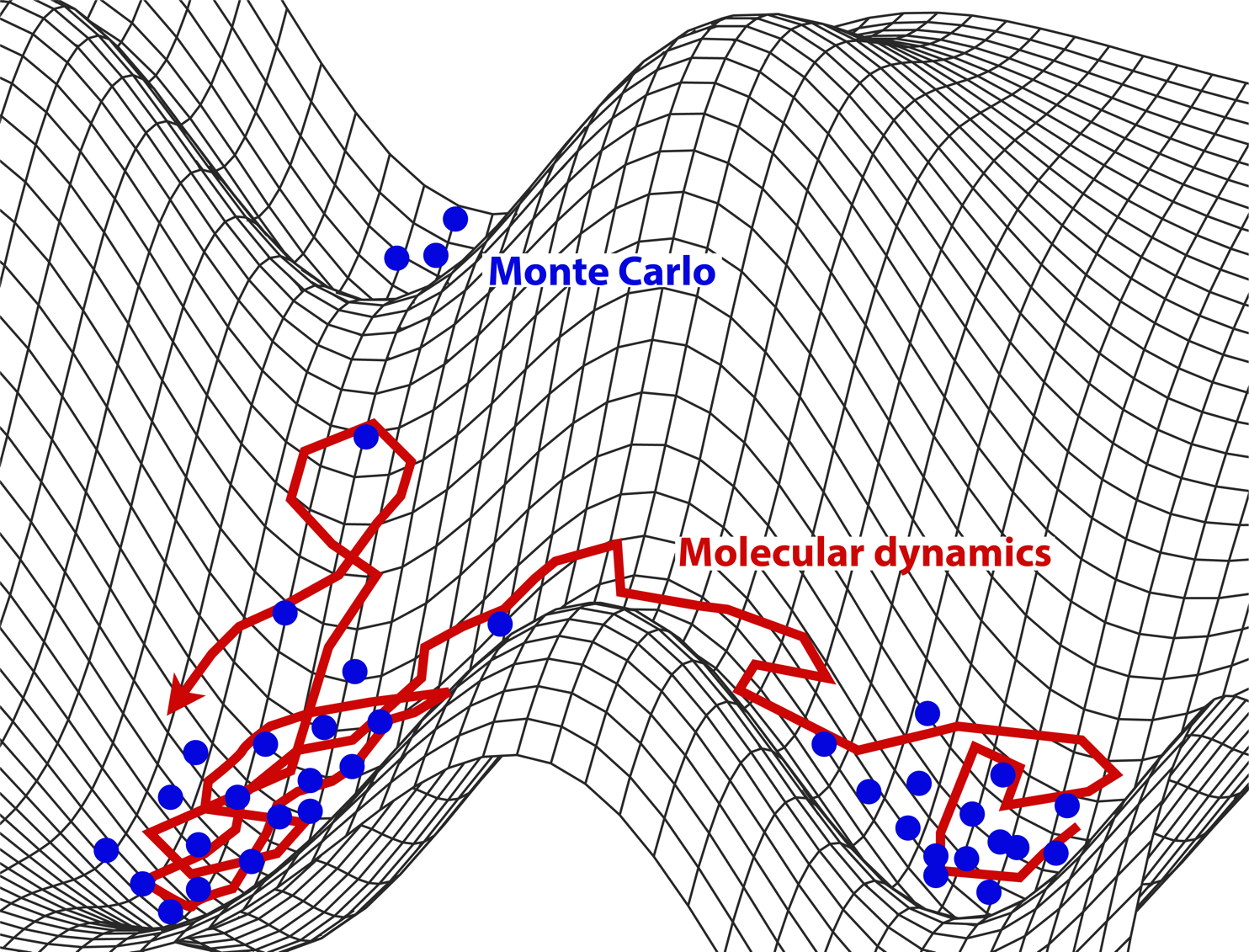
MD vs MC: Both sample microstates. The former follows the natural motion (dynamics); the latter samples from the Boltzmann distribution using rules designed to improve efficiency.
Timescales and Lengthscales
Classical molecular dynamics can access a hierarchy of time-scales from pico seconds to microseconds.
It is also possible to go beyond the time scale of brute-force MD by emplying clever enhanced sampling techniques.
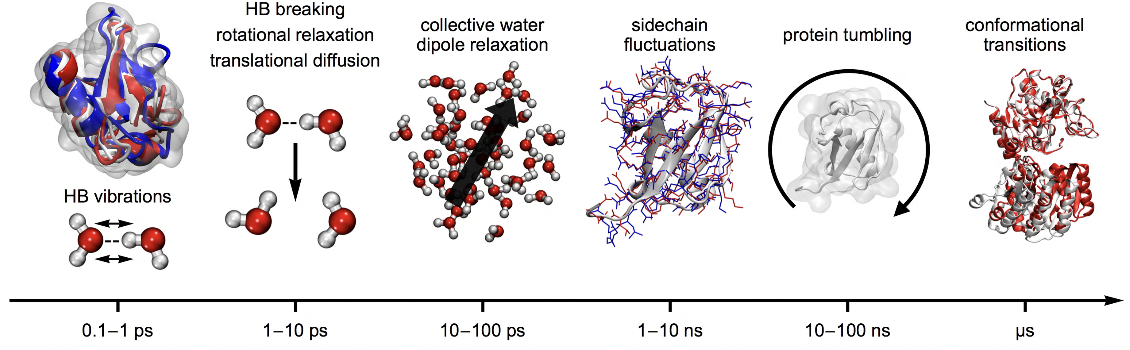
Different time-scales underlying different length-scales/motions in molecules
Simulation of water box
Is MD just Newton’s laws applied on big systems?
Not quite: Nobel Prize in Chemistry 2013
Classical molecular dynamics (MD) is a powerful computational technique for studying complex molecular systems.
Applications span wide range including proteins, polymers, inorganic and organic materials.
Also, molecular dynamics simulation is being used in a complementary way to the analysis of experimental data coming from NMR, IR, UV spectroscopies and elastic-scattering techniques, such as small angle scattering or diffraction.
Integrating equations of motion Numerically
The Euler method is the simplest numerical integrator for ordinary differential equations (ODEs).
More accurate integrators that include higher-order terms are known as Runge-Kutta (RK) methods — e.g., RK2, RK4, RK6.
Given an ODE in standard form:
we approximate the derivative using finite differences:
leading to the Euler update rule:
Example: Harmonic Oscillator
The harmonic oscillator with parameters is defined by the state vector with components for given by:
Using the Euler method, the system evolves as:
Source
import numpy as np
import matplotlib.pyplot as plt

y  = np.array([1.0, 1.0])  # Initial [x, v]
pos, vel = [], []
t  = 0
dt = 0.1

for i in range(1000):

    dydt = np.array([y[1], -y[0]])  # [v, -x]
    y += dt * dydt                  # Euler update

    t += dt

    pos.append(y[0])
    vel.append(y[1])

# Convert to arrays
pos, vel = np.array(pos), np.array(vel)

# Plot results
fig, ax = plt.subplots(ncols=3, nrows=1, figsize=(8,3))

# Phase space
ax[0].plot(pos, vel)
ax[0].set_title("Phase space (x vs v)")

# Time series
ax[1].plot(pos, label="x(t)")
ax[1].plot(vel, label="v(t)")
ax[1].legend()
ax[1].set_title("Time evolution")

# Energy
ax[2].plot(0.5*pos**2 + 0.5*vel**2)
ax[2].set_title("Energy (should be constant)")

plt.tight_layout()
plt.show()
Energy is not constant. The right-hand panel shows the energy growing steadily in time — a classic failure of Euler’s method. The reason is geometric: Euler is not symplectic, so the area in phase space (and hence the energy of an oscillator) is not preserved. Energy drift accumulates as over a simulation of length — for any choice of the drift will eventually dominate.
The fix is to use an integrator that respects the Hamiltonian structure — the Verlet family below.
Verlet algorithm
In 1967 Loup Verlet introduced a new algorithm into molecular dynamics simulations which preserves energy is accurate and efficient.
Summing the two taylor expansion above we get a updating scheme which is an order of mangnitude more accurate
Velocity is not needed to update the positions. But we still need them to set the temperature.
Terms of order cancel in position giving position an accuracy of order
To update the position we need positions in the past at two different time points! This is is not very efficient.
Velocity Verlet updating scheme
A better updating scheme has been proposed known as Velocity-Verlet (VV) which stores positions, velocities and accelerations at the same time. Time stepping backward expansion and summing with the forward Tayloer expansions we get Velocity Verlet updating scheme:
Molecular Dynamics of Classical Harmonic Oscillator (NVE)
Velocity Verlet integration of harmonic oscillator
Source
import numpy as np

def run_md_nve_1d(x, v, dt, t_max, en_force):
    """
    Minimalistic 1D Molecular Dynamics simulation (NVE ensemble)
    using Velocity Verlet integration.
    Simulates a particle moving in a 1D potential without thermal noise or friction
    (i.e., energy-conserving dynamics).

    Parameters
    ----------
    x : float
        Initial position.
    v : float
        Initial velocity.
    dt : float
        Time step for integration.
    t_max : float
        Total simulation time.
    en_force : callable
        Function that takes position `x` as input and returns a tuple (potential energy, force).

    Returns
    -------
    pos : ndarray
        Array of particle positions over time.
    vel : ndarray
        Array of particle velocities over time.
    KE : ndarray
        Array of kinetic energies over time.
    PE : ndarray
        Array of potential energies over time.

    Example
    -------
    >>> def harmonic_force(x):
    >>>     k = 1.0
    >>>     return 0.5 * k * x**2, -k * x
    >>> pos, vel, KE, PE = run_md_nve_1d(1.0, 0.0, 0.01, 10.0, harmonic_force)
    """

    times, pos, vel, KE, PE = [], [], [], [], []

    # Initialize force and potential energy
    pe, F = en_force(x)

    t = 0.0
    for step in range(int(t_max / dt)):

        # Velocity Verlet Integration

        # Half-step velocity update
        v += 0.5 * F * dt

        # Full-step position update
        x += v * dt

        # Update force at new position
        pe, F = en_force(x)

        # Half-step velocity update
        v += 0.5 * F * dt

        # Save results
        times.append(t)
        pos.append(x)
        vel.append(v)
        KE.append(0.5 * v * v)
        PE.append(pe)

        # Advance time
        t += dt

    return np.array(pos), np.array(vel), np.array(KE), np.array(PE)
Euler vs. Velocity Verlet: energy drift in numbers
To make the contrast quantitative, run both integrators on the same harmonic oscillator with the same time step and plot the relative energy error . Velocity-Verlet keeps the error bounded — it oscillates around a constant — while Euler’s error grows exponentially.
def run_euler_1d(x, v, dt, t_max, en_force):
    n = int(t_max / dt)
    pos, vel, KE, PE = np.zeros(n), np.zeros(n), np.zeros(n), np.zeros(n)
    for i in range(n):
        pe, F = en_force(x)
        # forward Euler
        x_new = x + dt * v
        v_new = v + dt * F
        x, v = x_new, v_new
        pos[i], vel[i], KE[i], PE[i] = x, v, 0.5 * v * v, pe
    return pos, vel, KE, PE


# Same parameters as the VV run
k_cmp, x0_cmp, v0_cmp = 3.0, 1.0, 0.0
dt_cmp = 0.05
t_max_cmp = 50.0

def ho_cmp(x, k=k_cmp):
    return k * x**2, -k * x

pE, vE, KEe, PEe = run_euler_1d(x0_cmp, v0_cmp, dt_cmp, t_max_cmp, ho_cmp)
pV, vV, KEv, PEv = run_md_nve_1d(x0_cmp, v0_cmp, dt_cmp, t_max_cmp, ho_cmp)

t_e = np.arange(len(pE)) * dt_cmp
t_v = np.arange(len(pV)) * dt_cmp
E0 = 0.5 * v0_cmp**2 + ho_cmp(x0_cmp)[0]
err_e = np.abs((KEe + PEe) - E0) / E0
err_v = np.abs((KEv + PEv) - E0) / E0

fig, ax = plt.subplots(figsize=(8, 4))
ax.semilogy(t_e, err_e, color='crimson', lw=1.5, label='Euler')
ax.semilogy(t_v, err_v, color='steelblue', lw=1.5, label='Velocity Verlet')
ax.set(xlabel='time', ylabel=r'$|E(t) - E(0)| / E(0)$',
       title=fr'Relative energy error  ($\Delta t = {dt_cmp}$)')
ax.legend()
ax.grid(True, ls=':', alpha=0.5, which='both')
fig.tight_layout()
Run NVE simulation of harmonic oscillator
Source
#----parameters of simulation----
k     = 3
x0    = 1
v0    = 0
dt    = 0.01 * 2*np.pi/np.sqrt(k) #A good timestep determined by using oscillator frequency
t_max = 1000

### Define Potential Energy function
def ho_en_force(x, k=k):
    '''Force field of harmonic oscillator:
    returns potential energy and force'''

    return k*x**2, -k*x

### Run simulation
pos, vel, KE, PE = run_md_nve_1d(x0, v0, dt, t_max, ho_en_force)

# Plot results
fig, ax = plt.subplots(ncols=3, nrows=1, figsize=(8,3))

# Phase space
ax[0].plot(pos, vel)
ax[0].set_title("Phase space (x vs v)")

# Time series
ax[1].plot(pos, label="x(t)")
ax[1].plot(vel, label="v(t)")
ax[1].legend()
ax[1].set_title("Time evolution")

# Energy
ax[2].plot(0.5*pos**2 + 0.5*vel**2)
ax[2].set_title("Energy (should be constant)")

plt.tight_layout()
plt.show()
Plot Distribution in phase-space
Source
### Visualize
fig, ax =plt.subplots(ncols=2)

ax[0].hist(pos);
ax[1].hist(vel, color='orange');
ax[0].set_ylabel('P(x)')
ax[1].set_ylabel('P(v)')

fig.tight_layout()
Ensemble averages
Langevin equation
A particle of mass moves under the force derived from a potential energy . The motion is purely deterministic.
Challenge: What should we do when we have only a one or few particles, and cannot explicitly simulate the vast surrounding environment in order to assign temperature?
Solution: We model the surrounding medium (e.g., a solvent) as an implicit thermal bath that interacts with the particle.
The particle exchanges energy with the bath, maintaining thermal equilibrium at a fixed temperature .
This motivates Langevin dynamics, where the effects of the solvent are captured by friction (dissipation) and random thermal kicks (fluctuations), without simulating solvent molecules explicitly.
The friction and thermal noise are clearly connected becasue the faster the particle movies (more noise) the more it also dissipates energy.
the connection is known by the name of Fluctuation-Dissipation Theorem:
The environment “forgets” what happened almost immediately after a collision very short memory hence noise terms are uncorrelated (independent). Just like what we had in brownian motion.
The FDT ensures that the strength of random thermal kicks is precisely tuned to the amount of viscous damping, so that the system reaches and maintains thermal equilibrium at temperature
FDT connects diffusion (random spreading) and viscosity (resistance to motion), both fundamentally controlled by temperature.
Derivation of FDT
We consider the underdamped Langevin equation for a free particle ():
Here:
is the velocity,
is the friction coefficient,
is Gaussian white noise with:
We want to compute the steady-state value of and relate it to , , and .
Step 1: Solve the Langevin Equation
We write the equation in standard ODE form:
This is a linear inhomogeneous ODE, solvable by integrating factor:
Step 2: Compute
We take the expectation:
This expands to:
The second term is zero since ,
For the third term, use the noise correlation:
Change variable:
So the full result is:
Long-Time Limit
As , the exponential terms vanish:
Apply Equipartition
At thermal equilibrium, equipartition gives:
Matching with the derived expression:
Molecular Dynamics of Harmonic oscillator (NVT)
Our goal is to numerically solve the Langevin equation:
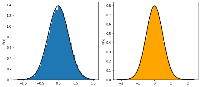
The target is to sample the canonical distribution:
There are many ways of integrating Langevin dynamics. The simplest is Euler-Maruyama (just like for diffusion), but it has poor accuracy and stability. We use the BAOAB scheme of Leimkuhler and Matthews, which splits the Langevin propagator into three pieces:
B: momentum kick by the conservative force, .
A: position drift (advance) at fixed velocity, .
O: Ornstein–Uhlenbeck step (friction + noise on velocity).
One BAOAB step alternates as B → A → O → A → B.
| Feature | Explanation |
|---|---|
| Stability | Handles both large and small friction robustly |
| Accuracy | Configurational averages are correct to |
| Efficiency | Allows large stable timesteps compared to naive Euler-Maruyama |
| Universality | Reduces to velocity-Verlet (Hamiltonian MD) at and to overdamped Langevin as |
Source
def langevin_md_1d(x, v, dt, kBT, gamma, t_max, en_force):
    '''Langevin dynamics applied to 1D potentials
    Using integration scheme known as BA-O-AB.
    INPUT: Any 1D function with its parameters
    '''

    times, pos, vel, KE, PE  = [], [], [], [], []

    t = 0
    for step in range(int(t_max/dt)):

        #B-step
        pe, F = en_force(x)
        v    += F*dt/2

        #A-step
        x += v*dt/2

        #O-step
        v = v*np.exp(-gamma*dt) + np.sqrt(1-np.exp(-2*gamma*dt)) * np.sqrt(kBT) * np.random.normal()

        #A-step
        x +=  v*dt/2

        #B-step
        pe, F = en_force(x)
        v    +=  F*dt/2

        ### Save output
        times.append(t), pos.append(x), vel.append(v), KE.append(0.5*v*v), PE.append(pe)

    return np.array(times), np.array(pos), np.array(vel), np.array(KE), np.array(PE)
Run Langevin dynamics of 1d harmonic oscillator
Source
import numpy as np
import matplotlib.pyplot as plt

# Initial conditions
x0 = 0.0
v0 = 0.5

# Input parameters
kBT   = 0.25
gamma = 0.01
dt    = 0.01
t_max = 10000
freq  = 10
k     = (2 * np.pi * freq)**2  # Spring constant (harmonic oscillator)

### Define Potential: Energy and Force
def ho_en_force(x, k=k):
    energy = 0.5 * k * x**2
    force  = -k * x
    return energy, force

### Langevin dynamics (assuming you have this function correctly defined)
# Should return arrays: times, pos, vel, KE, PE
times, pos, vel, KE, PE = langevin_md_1d(x0, v0, dt, kBT, gamma, t_max, ho_en_force)

### Plotting
fig, ax = plt.subplots(nrows=1, ncols=4, figsize=(10, 4))

bins = 50

# Theoretical distributions
def gaussian_x(x, k, kBT):
    return np.exp(-k*x**2/(2*kBT)) / np.sqrt(2*np.pi*kBT/k)

def gaussian_v(v, kBT):
    return np.exp(-v**2/(2*kBT)) / np.sqrt(2*np.pi*kBT)

# Plot histograms
ax[0].hist(pos, bins=bins, density=True, alpha=0.6, color='skyblue')
ax[1].hist(vel, bins=bins, density=True, alpha=0.6, color='salmon')

# Plot theoretical curves
x_grid = np.linspace(min(pos), max(pos), 300)
v_grid = np.linspace(min(vel), max(vel), 300)

ax[0].plot(x_grid, gaussian_x(x_grid, k, kBT), 'k-', lw=2, label='Theory')
ax[0].set_xlabel('Position x')
ax[0].set_ylabel('P(x)')
ax[0].legend()


ax[1].plot(v_grid, gaussian_v(v_grid, kBT), 'k-', lw=2, label='Theory')
ax[1].set_xlabel('Velocity v')
ax[1].set_ylabel('P(v)')
ax[1].legend()

ax[2].plot(pos[-1000:], vel[-1000:], alpha=0.3)
ax[2].set_xlabel('Position x')
ax[2].set_ylabel('Velocity v')
ax[2].set_title('Phase Space')

E_tot=KE+PE
ax[3].plot(E_tot)
ax[3].set_xlabel('Time')
ax[3].set_ylabel('Energy')
ax[3].set_title('Total Energy')

fig.tight_layout()
plt.show()
Double well potential
Source
def double_well(x, k=1, a=3):

    energy = 0.25*k*((x-a)**2) * ((x+a)**2)
    force = -k*x*(x-a)*(x+a)

    return energy, force

x = np.linspace(-6,6,1000)
energy, force = double_well(x)

plt.plot(x, energy, '-o',lw=3)
plt.plot(x, force, '-', lw=3, alpha=0.5)

plt.ylim(-20,40)
plt.grid(True)
plt.legend(['$U(x)$', '$F=-\partial_x U(x)$'], fontsize=15)Source
# Potential
def double_well(x, k=1, a=3):

    energy = 0.25*k*((x-a)**2) * ((x+a)**2)
    force = -k*x*(x-a)*(x+a)

    return energy, force

# Initial conditions
x     = 0.1
v     = 0.5

# Input parameters of simulation
kBT   = 5 # vary this
gamma = 0.1 # vary this
dt    = 0.05
t_max = 10000
freq  = 10

#### Run the simulation
times, pos, vel, KE, PE = langevin_md_1d(x, v, dt, kBT, gamma, t_max, double_well)

#### Plotting
fig, ax =plt.subplots(nrows=1, ncols=2, figsize=(13,5))

x = np.linspace(min(pos), max(pos), 50)

ax[0].plot(pos)
ax[1].hist(pos, bins=50, density=True, alpha=0.5);

v = np.linspace(min(vel), max(vel),50)

ax[0].set_xlabel('t')
ax[0].set_ylabel('x(t)')

ax[1].set_xlabel('Computed P(x)')
ax[1].set_ylabel('x')
Problems
Time step and stability. Run the velocity-Verlet harmonic oscillator (
run_md_nve_1d) with . Plot the relative energy error vs. time on log axes. Where does the integrator become unstable? Why is the criterion universal for explicit symplectic integrators?Boltzmann sampling. Run the Langevin harmonic oscillator at , for . Histogram the position trace and overlay the analytical Gaussian . Check that the variance equals — equipartition.
Friction limits. For the same harmonic oscillator, vary at fixed and . Plot vs. simulation time. Which equilibrates fastest? Which is closest to underdamped (oscillatory) vs. overdamped (purely diffusive)?
Custom 1D potential. Implement Langevin dynamics for . Try (a) a symmetric double well , (b) an asymmetric well . In each case histogram and overlay — do they agree? How does the agreement depend on the simulation length and on ?
Reference
B. Leimkuhler and C. Matthews, Robust and efficient configurational molecular sampling via Langevin dynamics, J. Chem. Phys. 138, 174102 (2013). Leimkuhler & Matthews (2013)
Additional learning resources:
UCSB ChE 210D — Principles of modern molecular simulation methods
D. Frenkel and B. Smit, Understanding Molecular Simulation: From Algorithms to Applications, 2nd ed. (Academic Press, 2002)
- Leimkuhler, B., & Matthews, C. (2013). Robust and efficient configurational molecular sampling via Langevin dynamics. The Journal of Chemical Physics, 138(17). 10.1063/1.4802990