Radial profiles of atomic orbitals
When visualizing the radial probabilities, it is possible to either directly plot the square of the radial wavefunction () or the radial probability density ():
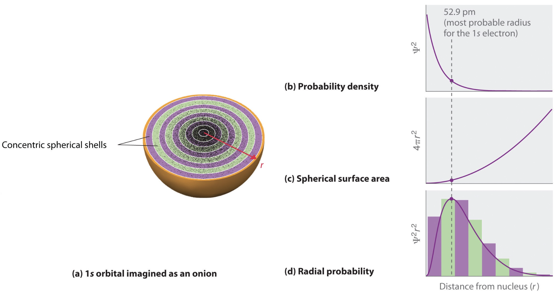
Fig.1 Radial probability density for several hydrogen orbitals. The peaks mark the most probable distance of the electron from the nucleus.
According to this expression, the most probable radius for an electron in the hydrogen-atom orbital is (the Bohr radius). The figure above shows examples of . Probability densities are useful, for example, in understanding charge distributions in atoms and molecules.
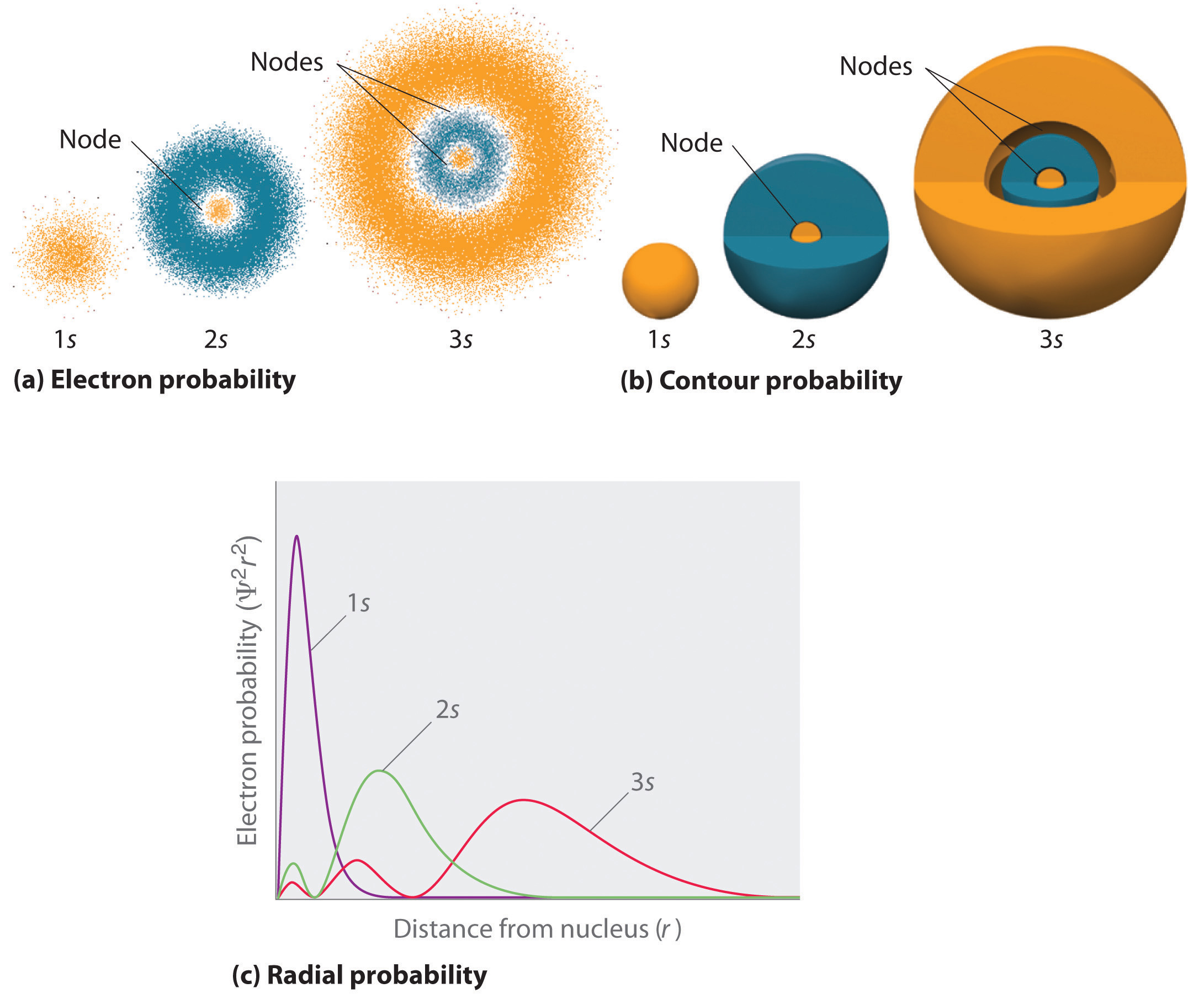
Fig.2 Radial wavefunctions and the associated radial probability densities for the lowest hydrogen orbitals.
As the principal quantum number increases, the electron moves out to greater distances from the nucleus. The average distance for an electron in a given orbital (with quantum numbers and ) is given by (this is not the same as the most probable value):
Note that the expectation value of and the most probable value of are not equal. The expectation value can be thought of like an average, and the most probable value like a maximum value.
3D shapes of orbitals
For degenerate states with , we have an additional degree of freedom in choosing how to represent the orbitals. In fact, any linear combination of a given set of orthogonal eigenfunctions corresponding to a degenerate set with orbital angular momentum is also a solution to the Schrödinger equation.
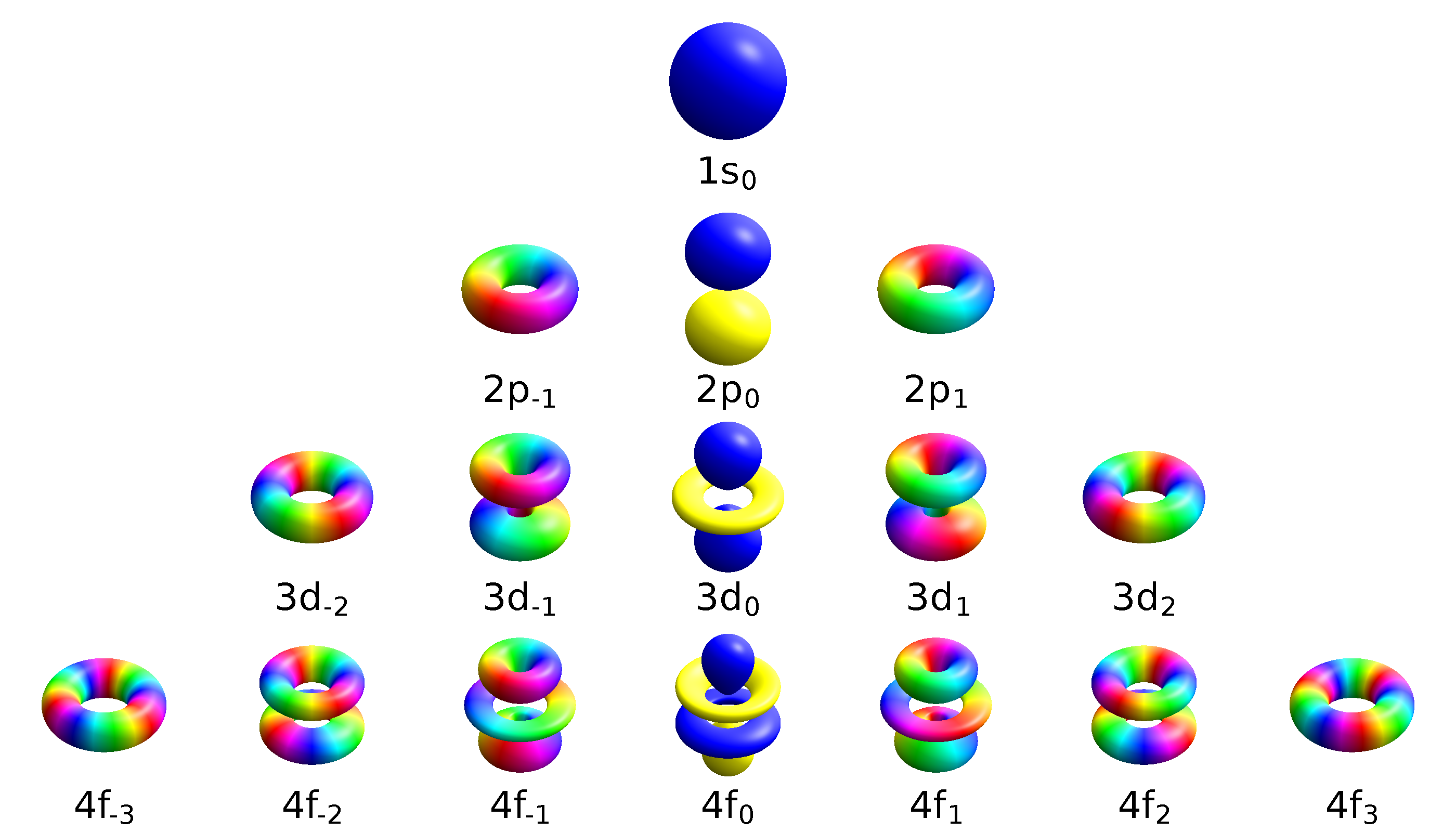
Fig.3 Shapes of the , , and atomic orbitals shown as isosurfaces of the probability density.
Two commonly used representations are the Cartesian form, which is real-valued (and, in the case of , denoted , , and ), and the eigenfunctions of angular momentum ( and ), which are complex-valued and denoted , , and . Both polar and Cartesian forms represent the same physical electron density, just in different coordinate frames. The relation between the representations is:
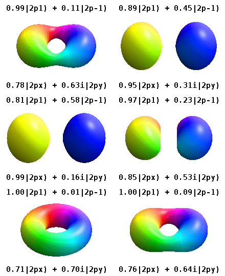
Fig.4 Animation showing how the complex orbitals and combine into the familiar real orbital.
By combining , , and , the lobe of the orbital can be made to point in any direction. For -orbitals, we have five degenerate levels:
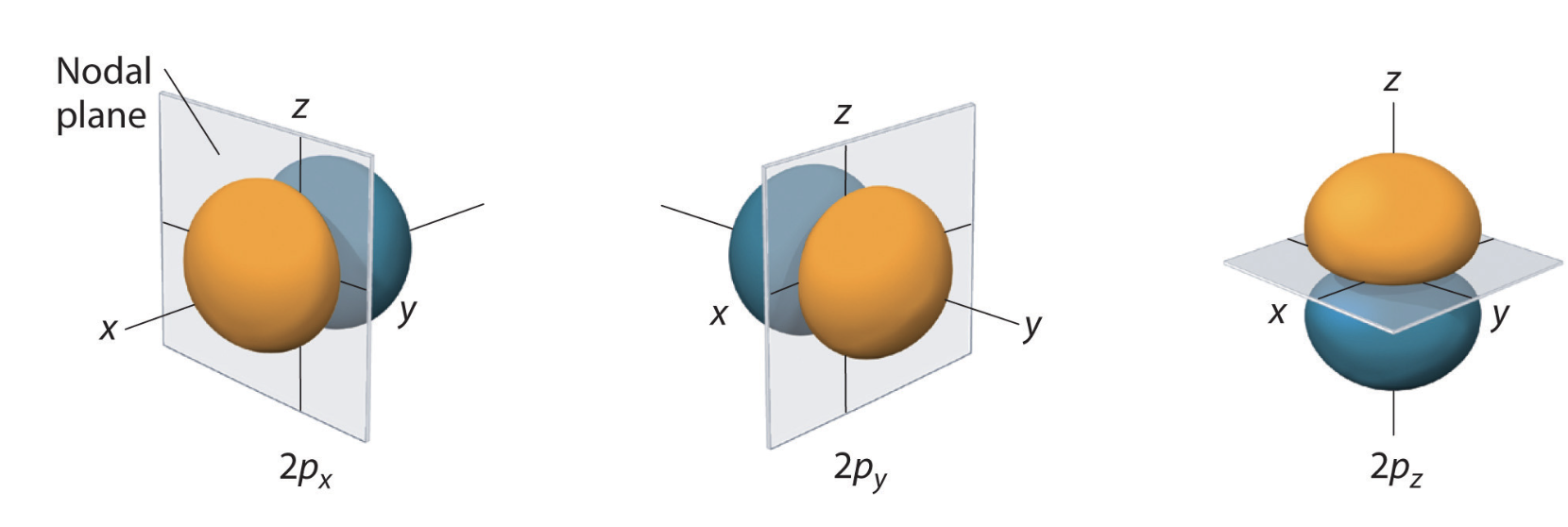
Fig.5 The three real orbitals (, , ) point along the Cartesian axes; their linear combinations can point in any direction.
Table of 2D orbitals
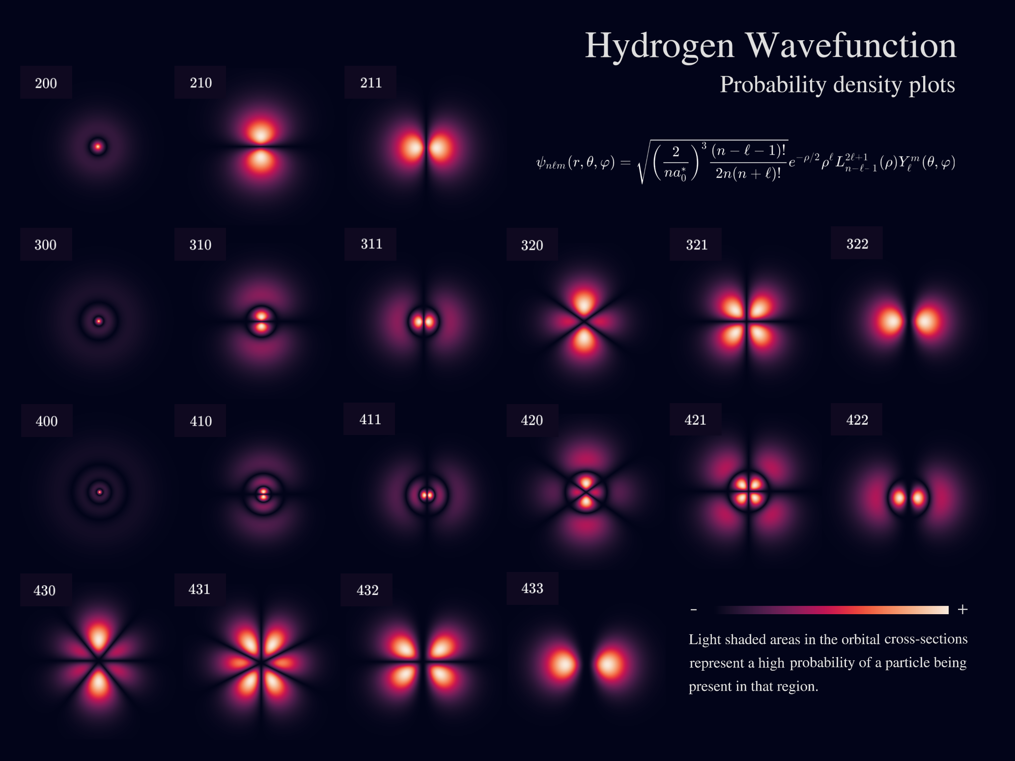
Fig.6 Two-dimensional cross sections of the probability densities for hydrogen orbitals.
Table of 3D orbitals
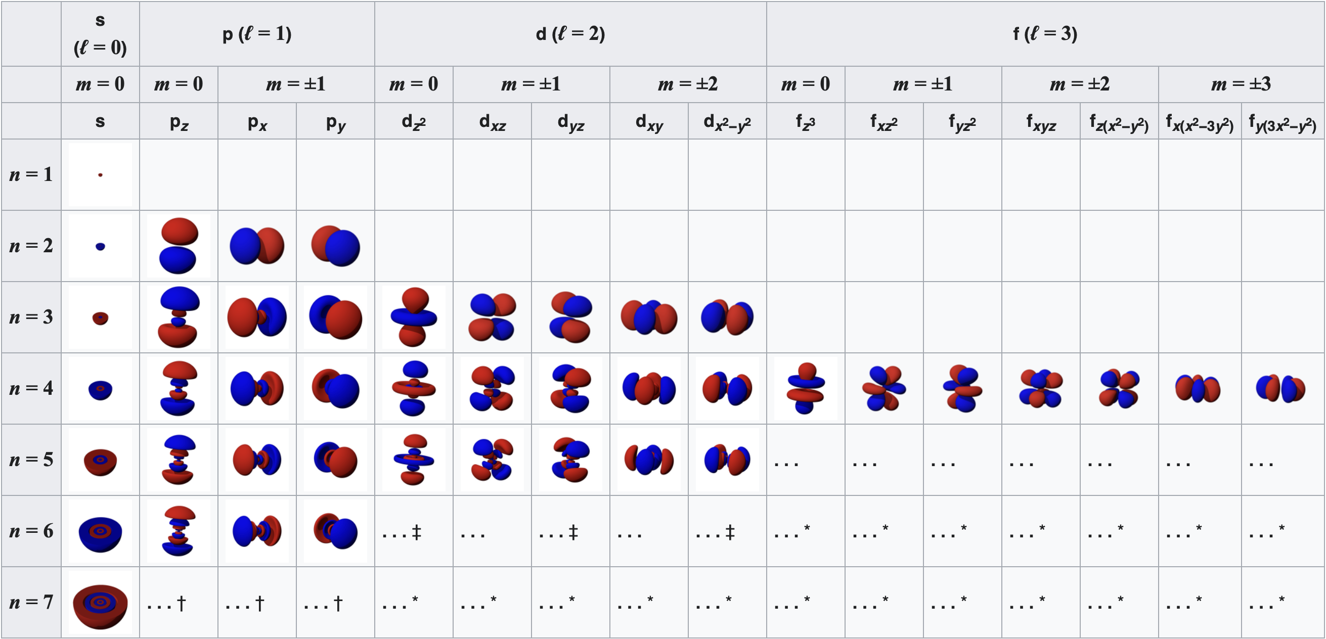
Fig.7 Three-dimensional isosurface renderings of hydrogen atomic orbitals.
Interactive plotter of atomic orbitals
Or build any orbital yourself; the menus only offer valid quantum numbers, and blue and red are the positive and negative lobes: