Electron Spin - Quantum Mechanics for Chemistry

What you will learn

Magnetism arises from the circular motion of charged particles.
Atoms with electrons that have nonzero orbital angular momentum generate magnetic moments, making them susceptible to the effects of an external magnetic field.
The Stern-Gerlach experiment established the existence of an intrinsic magnetic moment in electrons, called spin, which is affected by a magnetic field independently of orbital angular momentum.
Despite the name, spin is an intrinsic magnetic property of subatomic particles and does not involve literal “spinning” or motion. Spin is a fundamental property of particles, akin to mass or charge.
Particles with half-integer spins (e.g., $1/2$ , $3/2$ , $5/2$ ) are classified as fermions, while those with integer spins (e.g., 0, 1, 2) are classified as bosons. These two families follow different rules. Fermions obey the Pauli exclusion principle, which states that no two identical fermions can occupy the same quantum state simultaneously. In contrast, bosons are not restricted in this way and can occupy the same state, allowing them to “bunch together.”
Normal Zeeman effect: the splitting of singlet states (spin zero) in a magnetic field due to the electron’s orbital angular momentum, which can be explained classically.
Anomalous Zeeman effect: a more general case where both electron spin and orbital angular momentum contribute to the splitting of energy levels in a magnetic field.

Rotating charge generates a magnetic moment¶

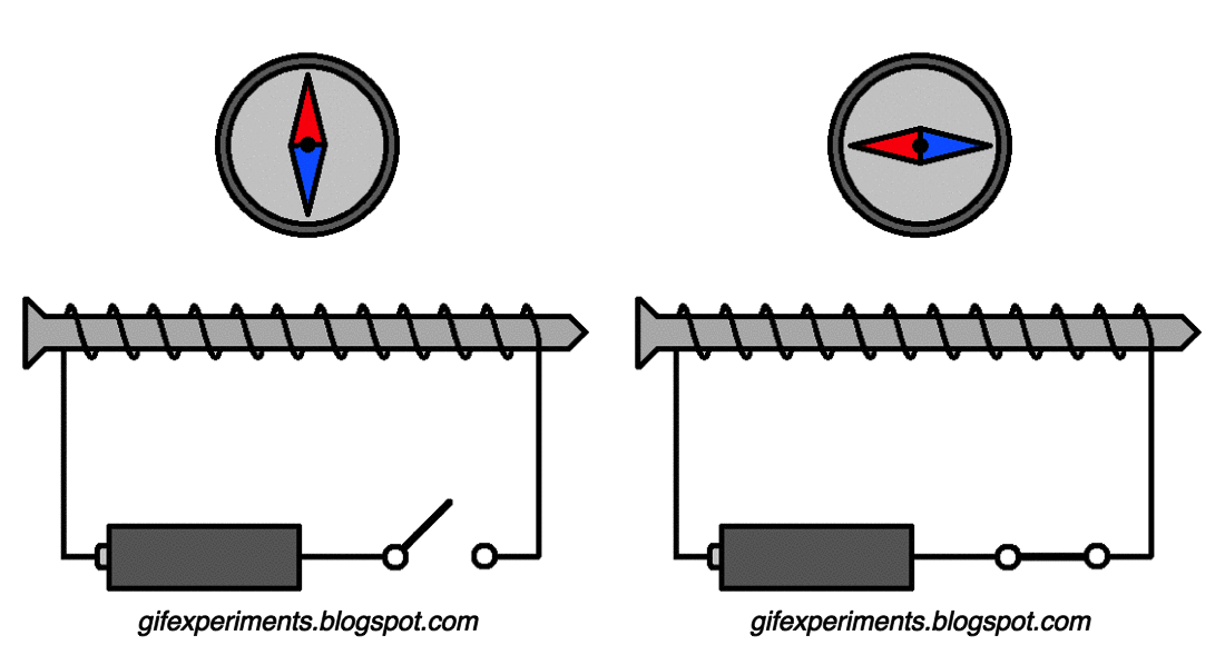
Magnetic field around a current-carrying wire — Fig.1 A magnetic field circulates around a current-carrying wire. A moving charge generates a magnetic moment.

A moving charge generates a magnetic moment, which interacts with an external magnetic field.
When an electron is in a state with $l > 0$ , one can picture a circular motion of charge (the wavefunction describing the electron) around the nucleus, generating its own magnetic field.
Note that this motion is not classical; here we are just building a wireframe picture based on a classical interpretation.

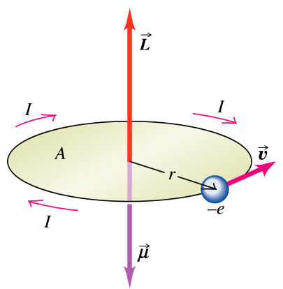
Magnetic moment and angular momentum of an orbiting charge — Fig.2 The magnetic moment and angular momentum generated by a charge moving on an orbit.

Magnetic moment of the electron¶

According to classical mechanics, a charged particle like an electron rotating around an axis has a magnetic moment given by:

{\vec{\mu} = \gamma_e\vec{L}}

(1)

where $\gamma_e$ is the magnetogyric ratio of the electron, expressed via fundamental constants as $-\frac{e}{2m_e}$ . We choose the external magnetic field to lie along the $z$ -axis, so it is the $z$ component of $\vec{\mu}$ that matters:

{\mu_z = -\left(\frac{e}{2m_e}\right)L_z = -\left(\frac{e\hbar}{2m_e}\right)m \equiv -\mu_B m}

(2)

where $\mu_B$ is the Bohr magneton. The interaction between a magnetic moment and an external magnetic field is given by the classical expression:

{U = -\vec{\mu}\cdot\vec{B} = -|\vec{\mu}||\vec{B}|\cos(\alpha)}

(3)

where $\alpha$ is the angle between the two vectors. This gives the energy for a bar magnet in the presence of an external field.

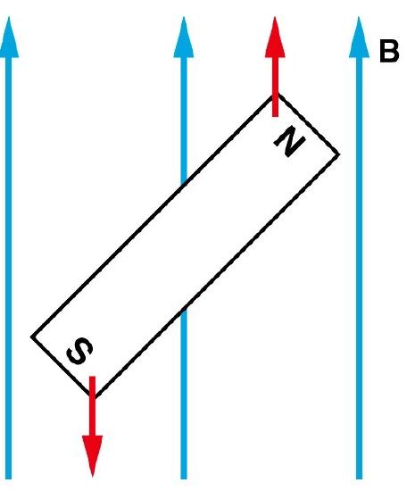
Torque on a magnet in an external field — Fig.3 An external magnetic field exerts a torque on a magnet. The interaction energy is proportional to the field strength $B$ and the magnetic moment $\mu$ .

Unlike in quantum mechanics, in classical mechanics any orientation is allowed. When the external field is oriented along the $z$ -axis, the classical potential energy of interaction with the field is:

{U = -\mu_z B = \frac{eB}{2m_e}L_z}

(4)

In quantum mechanics, to get the Hamiltonian term for interaction with the magnetic field, we simply replace the classical angular momentum with the corresponding operator:

\hat{H}_{mag} = \frac{eB}{2m_e}\hat{L}_z

(5)

Effect of a magnetic field on atoms¶

In quantum mechanics, a magnetic moment (here corresponding to a non- $s$ orbital electron) may only take specific orientations.
The $z$ -axis is often called the quantization axis. The eigenvalues of $\hat{L}_z$ give the possible orientations of the magnetic moment with respect to the external field.
For example, consider an electron in a $2p$ orbital of a hydrogenlike atom. The electron may reside in any of $2p_{+1}$ , $2p_0$ , or $2p_{-1}$ (degenerate without the field). For these orbitals $L_z$ may take the values $+\hbar$ , 0, $-\hbar$ :

{\hat{L}_z|p_{+1}\rangle = +1\times\hbar|p_{+1}\rangle}

(6)

{\hat{L}_z|p_0\rangle = 0\times\hbar|p_{0}\rangle}

(7)

{\hat{L}_z|p_{-1}\rangle = -1\times\hbar|p_{-1}\rangle}

(8)

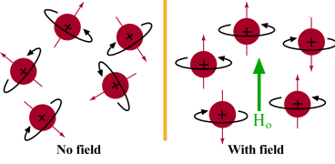
External field orienting atomic magnetic moments — Fig.4 An external magnetic field orients atoms with dipole moments due to electrons in nonzero- $l$ orbitals.

A magnetic field modifies the Hamiltonian¶

The total quantum mechanical Hamiltonian for a hydrogenlike atom in a magnetic field can be written as:

{\hat{H} = \hat{H}_0 + \frac{eB}{2m_e}\hat{L}_z}

(9)

where $\hat{H}_0$ denotes the Hamiltonian in the absence of the magnetic field.
Since the projection of angular momentum commutes with the Hamiltonian, $[\hat{L}_z, \hat{H}_0] = 0$ , both operators share the same eigenfunctions:

\hat{L}_z \mid n,l, m_l\rangle = \hbar m_l \mid n,l, m_l\rangle

(10)

\hat{H}_0 \mid n,l, m_l\rangle = E_n \mid n,l, m_l\rangle

(11)

Zeeman effect¶

We see that the magnetic field now enters the expression for the energy levels.
The field splits the $(2l + 1)$ degenerate levels. This is called the orbital Zeeman effect.
For instance, the $2p$ level of the hydrogen atom splits into 3 levels at energies $-\mu_B B$ , 0, $+\mu_B B$ .

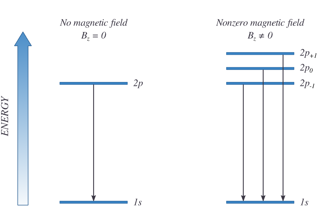
Zeeman splitting of the 2p level — Fig.5 The Zeeman effect: when an external magnetic field is applied, sharp spectral lines of hydrogen split into multiple closely spaced lines. Shown is the splitting of the degenerate $2p$ level into three states differing in $m_l = -1, 0, +1$ .

Discovering spin¶

Spin as a tiny magnet¶

We come to view the spin of subatomic particles in the same way as mass and charge. Spin is an intrinsic property of subatomic particles like protons, electrons, and photons.
Spin manifests itself via a permanent magnetic moment. A particle with spin can interact with magnetic fields just as a charged particle interacts with electric fields. This is why spin is pictorially depicted as a tiny magnet.

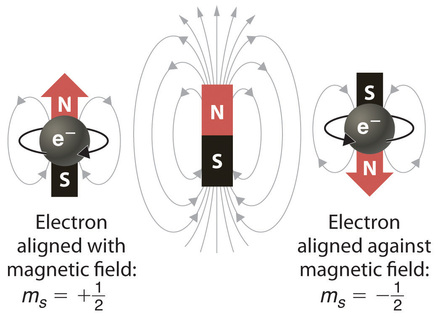
Spin pictured as a tiny magnet — Fig.6 Spin is pictured as a tiny permanent magnet associated with each particle.

The Schrödinger equation does not naturally account for electron spin. This is because spin lacks a classical analogue, so our approach of taking the classical Hamiltonian and replacing terms with operators does not work directly for spin.
The concept of electron spin originates from the Dirac equation, which is essentially a generalization of the Schrödinger equation to include relativistic effects.
Fortunately, spin can be incorporated into the Schrödinger equation once we recognize its existence. We simply add an additional quantum number, $s$ , which behaves similarly to the orbital angular momentum $l$ .

Quantum numbers and eigenfunctions of spin¶

Spin and its projection, $S$ and $S_z$ , have the same properties as the angular momentum $L$ and $L_z$ . Quantum mechanics requires the number of allowed spin projections to be:

2s + 1

(13)

Experiments show that we only observe two values of spin:

2s + 1 = 2 \quad \Rightarrow \quad s = \frac{1}{2}

(14)

Projections are determined by the quantum number $m_s$ , an analog of $m_l$ :

m_s = -s, +s = -1/2, +1/2

(15)

We expect two eigenfunctions for the two outcomes and denote the eigenfunctions of $S_z$ as $\alpha$ and $\beta$ :

Eigenfunctions of spin, $\alpha$ and $\beta$

Spin is an intrinsic angular momentum with a fixed eigenvalue:

S = \frac{\sqrt{3}}{2}\hbar

(16)

S_z = \pm \frac{1}{2}\hbar

(17)

Spin eigenfunctions and eigenvalues:

\hat{S}^2 |\alpha\rangle = \hbar^2 s(s+1) |\alpha\rangle = \frac{3}{4} \hbar^2 |\alpha\rangle

(18)

\hat{S}^2 |\beta\rangle = \hbar^2 s(s+1) |\beta\rangle = \frac{3}{4} \hbar^2 |\beta\rangle

(19)

\hat{S}_z |\alpha\rangle = +\frac{1}{2} \hbar |\alpha\rangle

(20)

\hat{S}_z |\beta\rangle = -\frac{1}{2} \hbar |\beta\rangle

(21)

Orthogonality and normalization of the spin part of the wavefunction¶

Note that the following operators commute: $\hat{H}$ , $\hat{L}^2$ , $\hat{L}_z$ , $\hat{S}^2$ , and $\hat{S}_z$ . This implies that all these quantities can be specified simultaneously.
The spin eigenfunctions $\alpha$ and $\beta$ are, as expected, orthonormal:

\int \alpha^* \alpha \, d\sigma \equiv \langle \alpha | \alpha \rangle = \int \beta^* \beta \, d\sigma \equiv \langle \beta | \beta \rangle = 1

(22)

\int \alpha^* \beta \, d\sigma \equiv \langle \alpha | \beta \rangle = \int \beta^* \alpha \, d\sigma \equiv \langle \beta | \alpha \rangle = 0

(23)

To completely describe a hydrogenlike atom, the wavefunction must include the spin component. Thus the total wavefunction is a product of the spatial wavefunction and the spin part:

|n,l, m_l, m_s\rangle = \psi_{n, l, m_l}(r, \theta, \phi)\,\sigma(s), \quad \text{where } \sigma = \alpha \text{ or } \beta

(24)

Wavefunctions differing in their spin part are orthogonal:

\langle 1, 0, 0, +1/2 \mid 1, 0, 0, -1/2\rangle = 0

(25)

Action of spin operators on eigenstates

In quantum mechanics the spin of an electron is represented by the spin operator $\vec{S}$ , with components $S_x$ , $S_y$ , and $S_z$ . For spin- $\frac{1}{2}$ particles, these operators are represented by the Pauli matrices $\sigma_x$ , $\sigma_y$ , and $\sigma_z$ (multiplied by $\frac{\hbar}{2}$ ):

S_x = \frac{\hbar}{2} \sigma_x, \quad S_y = \frac{\hbar}{2} \sigma_y, \quad S_z = \frac{\hbar}{2} \sigma_z

(26)

The Pauli matrices are:

\sigma_x = \begin{pmatrix} 0 & 1 \\ 1 & 0 \end{pmatrix}, \quad \sigma_y = \begin{pmatrix} 0 & -i \\ i & 0 \end{pmatrix}, \quad \sigma_z = \begin{pmatrix} 1 & 0 \\ 0 & -1 \end{pmatrix}

(27)

The spin eigenstates $\alpha$ and $\beta$ correspond to “spin-up” and “spin-down” along the $z$ -axis:

\alpha = \begin{pmatrix} 1 \\ 0 \end{pmatrix}, \quad \beta = \begin{pmatrix} 0 \\ 1 \end{pmatrix}

(28)

$S_z$ operator:

S_z \alpha = \frac{\hbar}{2} \begin{pmatrix} 1 & 0 \\ 0 & -1 \end{pmatrix} \begin{pmatrix} 1 \\ 0 \end{pmatrix} = \frac{\hbar}{2} \alpha

(29)

S_z \beta = \frac{\hbar}{2} \begin{pmatrix} 1 & 0 \\ 0 & -1 \end{pmatrix} \begin{pmatrix} 0 \\ 1 \end{pmatrix} = -\frac{\hbar}{2} \beta

(30)

$S_x$ operator:

S_x \alpha = \frac{\hbar}{2} \begin{pmatrix} 0 & 1 \\ 1 & 0 \end{pmatrix} \begin{pmatrix} 1 \\ 0 \end{pmatrix} = \frac{\hbar}{2} \beta

(31)

S_x \beta = \frac{\hbar}{2} \begin{pmatrix} 0 & 1 \\ 1 & 0 \end{pmatrix} \begin{pmatrix} 0 \\ 1 \end{pmatrix} = \frac{\hbar}{2} \alpha

(32)

$S_y$ operator:

S_y \alpha = \frac{\hbar}{2} \begin{pmatrix} 0 & -i \\ i & 0 \end{pmatrix} \begin{pmatrix} 1 \\ 0 \end{pmatrix} = \frac{i \hbar}{2} \beta

(33)

S_y \beta = \frac{\hbar}{2} \begin{pmatrix} 0 & -i \\ i & 0 \end{pmatrix} \begin{pmatrix} 0 \\ 1 \end{pmatrix} = -\frac{i \hbar}{2} \alpha

(34)

Summary table

Operator	$\alpha$ (spin-up)	$\beta$ (spin-down)
$S_z$	$\frac{\hbar}{2} \alpha$	$-\frac{\hbar}{2} \beta$
$S_x$	$\frac{\hbar}{2} \beta$	$\frac{\hbar}{2} \alpha$
$S_y$	$\frac{i \hbar}{2} \beta$	$-\frac{i \hbar}{2} \alpha$

Magnetic moment due to spin¶

Analogously, the $\hat{S}_x$ and $\hat{S}_y$ operators can be defined. These do not commute with $\hat{S}_z$ . Because electrons have spin angular momentum, the unpaired electrons in silver atoms (Stern-Gerlach experiment) produce an overall magnetic moment (the “two spots” of silver atoms). The spin magnetic moment is proportional to the spin angular momentum:

{\vec{\hat{\mu}}_S = -\frac{g_e e}{2m_e}\vec{\hat{S}}}

(35)

where $g_e$ is the free-electron $g$ -factor (2.002322 from quantum electrodynamics). The $z$ -component of the spin magnetic moment is ( $z$ is the quantization axis):

The Hamiltonian depends on the spin operator¶

Following the eigenfunctions of $S_z$ obtained above, the corresponding eigenvalues for the spin magnetic moment are:

{\mu_z = -\frac{g_e e\hbar}{2m_e}m_s = -g_e\mu_B m_s}

(37)

Thus the total energy for a spin in an external magnetic field is:

{E = g_e\mu_B m_s B}

(38)

where $B$ is the magnetic field strength (in tesla). By combining the contributions from the hydrogenlike-atom Hamiltonian and the orbital and electron Zeeman terms, we get the total Hamiltonian:

{\hat{H} = \hat{H}_0 + \frac{eB}{2m_e}\hat{L}_z + \frac{g_e eB}{2m_e}\hat{S}_z = \hat{H}_0 + \frac{eB}{2m_e}\left(\hat{L}_z + g_e\hat{S}_z\right)}

(39)

The eigenvalues of this operator are (derivation not shown):

{E_{n,m_l,m_s} = E_n + \frac{eB\hbar}{2m_e}\left(m_l + g_e m_s\right)}

(40)

Spin-orbit coupling¶

Having two sources of magnetic field in atoms, one due to orbital momentum and another due to spin, there arises the possibility that these microscopic magnets can interact.
This possibility is indeed realized and is known as spin-orbit coupling. A new term is added to the Hamiltonian to account for it:

\hat{H} = \hat{H}_0 + \frac{A}{r^3} \cdot \hat{L}\cdot\hat{S}

(41)

where $A$ is a constant, $\hat{H}_0$ is the Hamiltonian for the H-atom without spin, and $\hat{L}$ and $\hat{S}$ are the orbital and spin angular momentum operators. Notice two things: first, the term decays as $1/r^3$ , faster than the potential energy, so this term makes a much smaller contribution than $\hat{H}_0$ .
Second, because of spin-orbit coupling, neither $\hat{L}$ nor $\hat{S}$ commutes with the Hamiltonian. Hence one needs a new quantum number $J$ to specify H-atom states. This new quantum number is the total angular momentum $\vec{J} = \vec{L} + \vec{S}$ .

Microstates from spin-orbit coupling for the 2p level — Fig.7 Determining the total angular momentum $j = l + s$ from the fact that projections add as $m_j = m_l + m_s$ and that $j$ follows angular-momentum quantization with $2j + 1$ values. Shown is the $l = 1$ state of hydrogen ( $2p^1$ ), which gives rise to the $^2P_{3/2}$ and $^2P_{1/2}$ microstates.

Determining total angular momentum values for the H-atom¶

Understand angular momentum coupling. In a hydrogen atom, the total angular momentum $\vec{J}$ is the vector sum of the orbital angular momentum $\vec{L}$ and the spin angular momentum $\vec{S}$ :

\vec{J} = \vec{L} + \vec{S}

(42)

Here $l$ is the orbital angular momentum quantum number ( $l = 0, 1, 2, \dots$ ) and $s$ is the spin quantum number ( $s = \frac{1}{2}$ for an electron).

Determine the possible $j$ values. The quantum number $j$ represents the magnitude of $\vec{J}$ and takes the values:

j = |l - s|, |l - s| + 1, \dots, (l + s)

(43)

Calculate $j$ based on $l$ and $s$ . Since $s = \frac{1}{2}$ for a single electron:

If $l = 0$ : $j = \frac{1}{2}$ only.
If $l = 1$ : $j = \frac{1}{2}$ and $j = \frac{3}{2}$ .
If $l = 2$ : $j = \frac{3}{2}$ and $j = \frac{5}{2}$ .
In general: $j = l \pm \frac{1}{2}$ .

Interpretation. These $j$ values correspond to the quantized total angular momentum. The magnitude is $|\vec{J}| = \sqrt{j(j+1)}\,\hbar$ . The $j$ values determine the energy-level splitting due to spin-orbit coupling (fine structure).

Term symbols¶

Because of spin-orbit coupling, the energy levels are no longer described by $l$ and $s$ separately. This is why one introduces term symbols, which encode the total spin multiplicity $(2S+1)$ , the angular momentum $L$ , and the total angular momentum $J = L + S$ . The word “total” takes on more meaning for multi-electron atoms, where angular momenta are summed. For the H-atom, $S = 1/2$ and $L = l$ :

^{2S+1}L_J

(44)

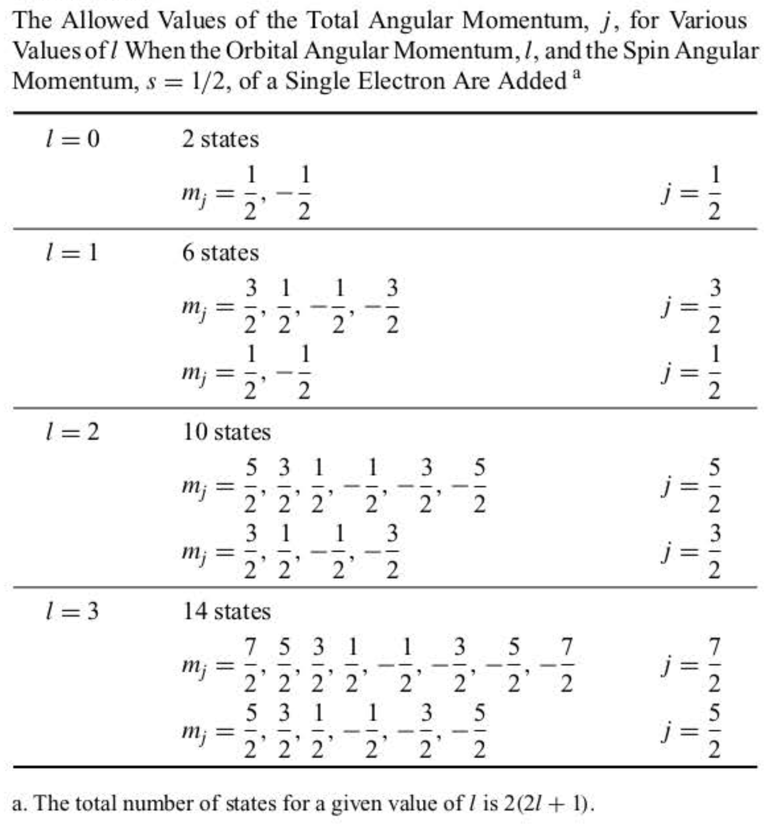
Allowed values of the total angular momentum j — Fig.8 Allowed values of the total angular momentum $j$ .

Solution:

The $j = l + s$ values follow the rules of spatial quantization of angular momentum, just like $l$ and $s$ : the projection of $J$ , namely $m_j$ , can take the values $l+s, l+s-1, \ldots, -(l+s)$ . Since $s = 1/2$ , we get $j = l + 1/2$ and $j = l - 1/2$ . The total number of microstates equals the 2 values of $m_s$ ( $+1/2, -1/2$ ) times the $2l+1$ values of $m_l$ , for a total of $2(2l+1)$ microstates.

For $l = 1$ : the maximum projection is $m_j = 1 + 1/2 = 3/2$ , coming from $j = 3/2$ ; the minimum is $m_j = l - 1/2 = 1/2$ , coming from $j = 1/2$ . We thus have two terms, $^2P_{3/2}$ and $^2P_{1/2}$ .

The “anomalous” Zeeman effect¶

While the Zeeman effect in some atoms (e.g., hydrogen) showed the expected equally spaced triplet, in other atoms the magnetic field split the lines into four, six, or even more lines, with some spacings wider than expected. These deviations were labeled the anomalous Zeeman effect and were very puzzling to early researchers.
The explanation gave additional insight into electron spin. With the inclusion of electron spin in the total angular momentum, the other multiplets fall into a consistent picture. So what has historically been called the “anomalous” Zeeman effect is really the normal Zeeman effect once electron spin is included.

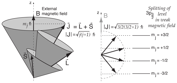
Splitting of spectral lines by m_J — Fig.9 In the presence of a magnetic field the spectral lines split further into levels described by $m_J$ .

When a magnetic field is applied to the H-atom, the external field $B$ now interacts with the total combined angular momentum $J$ , splitting the energy of each level with distinct $J$ . For example, $^2P_{3/2}$ splits into $2\cdot 3/2 + 1 = 4$ lines and $^2P_{1/2}$ splits into $2\cdot 1/2 + 1 = 2$ lines.

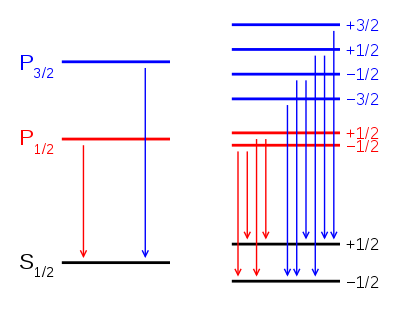
Anomalous Zeeman effect energy diagram — Fig.10 Anomalous Zeeman effect. (Left) Spectral lines split into multiple microstates because of spin-orbit coupling; states are described by term symbols. (Right) With a weak magnetic field the lines split further according to the values of $j$ and its projection $m_j$ .

Selection rules for electronic transitions¶

Just as for other model systems, the probability of an electronic transition in the H-atom is given by the transition moment (or its $z$ -projection), $\langle n', l', m_l', m_s' \mid z \mid n, l, m_l, m_s \rangle$ . Evaluating this expression using the properties of the special functions yields the following selection rules.

Summary of spin and angular momentum¶

Spin emerges naturally once one accounts for relativistic effects, as originally shown by Paul Dirac. Except in special cases, relativistic effects are not significant enough to include in quantum mechanics, so we incorporate spin as an additional degree of freedom that has not been accounted for but is known to exist.

Angular momentum	Spin momentum
$\hat{L} = \hat{r}\times \hat{p}$ $\hat{L}_z = -i\hbar \left(x\frac{\partial}{\partial y} - y\frac{\partial}{\partial x}\right)$	$\hat{S}$ $\hat{S}_z$
$l = 0, 1, 2, 3, ...$ $m_l = -l...0...l$	$s = 1/2$ $m_s = -1/2, 1/2$
$\mid l, m_l\rangle = Y_{l, m_l}$	$\mid s, m_s\rangle = \alpha, \beta$ $\mid 1/2, +1/2\rangle = \alpha$ $\mid 1/2, -1/2\rangle = \beta$
$L = \hbar\sqrt{l(l+1)}$ $L_z = \hbar m_l$	$S = \hbar\sqrt{s(s+1)} = \hbar\sqrt{3/4}$ $S_z = \hbar m_s = \pm \hbar/2$
$\mu_L = -g_l \frac{e}{2m_e}L$ $g_l = 1$	$\mu_S = g_s \frac{e}{2m_e}S$ $g_s \approx 2$

Problems¶

These problems span the whole chapter, from hydrogen orbitals and their quantum numbers to electron spin, Zeeman splitting, and spin-orbit coupling.

Problem 1: Counting states for $n = 3$

For the hydrogen atom, how many possible quantum states correspond to the principal quantum number $n = 3$ ?
What are the energies of these states?
Consider several values of $n$ and show that the number of orbitals for each $n$ is $n^2$ .

Solution:

If $n = 3$ , the allowed values of $l$ are 0, 1, and 2.

If $l = 0$ , then $m = 0$ (1 state).
If $l = 1$ , then $m = -1, 0, 1$ (3 states).
If $l = 2$ , then $m = -2, -1, 0, 1, 2$ (5 states).

In total there are $1 + 3 + 5 = 9$ allowed states. This confirms that the number of orbitals for the H-atom is $n^2$ .

Because the total energy depends only on the principal quantum number $n = 3$ , the energy of each of these states is:

E_n = -13.6 \cdot \frac{1}{n^2} \, [\text{eV}]

(48)

Problem 2: Nodes of the $3p_z$ orbital

Locate the nodes (and nodal surfaces) of the $3p_z$ orbital:

\psi_{3p_z} = \frac{1}{81}\sqrt{\frac{2}{\pi}}\left(\frac{1}{a_0}\right)^{3/2}\left(6\frac{r}{a_0} - \frac{r^2}{a_0^2}\right) e^{-r/3a_0}\cos(\theta)

(49)

Solution:

$3p_z$ corresponds to $n = 3$ , $l = 1$ , and $m_l = 0$ .
The radial part is zero at $r = 0$ and $r = 6a_0$ . The first is part of the boundary condition and not a node, because the wavefunction does not change sign there. Hence there is 1 radial node.
The angular part has one nodal surface from $\cos\theta = 0$ , which occurs at $\theta = \frac{\pi}{2}$ (the $xy$ -plane).
We thus have 2 nodes for the $3p_z$ orbital. The total number of nodes is $n - 1$ , made up of $l$ angular nodes and $n - l - 1$ radial nodes.