Wave equation

What you will learn

The wave equation $u_{xx} = u_{tt}/v^2$ is a linear second-order PDE. Any sum of solutions is again a solution, so the general solution can be assembled from simple building blocks.
Boundary conditions (what the wave does at the edges) and initial conditions (its shape and velocity at $t=0$ ) turn the general solution into the one solution that describes a particular system.
Separation of variables, $u(x,t)=X(x)T(t)$ , splits the PDE into two ordinary differential equations that we solve with an exponential trial function.
Fixed ends quantize. For a string of length $L$ the boundary conditions allow only the normal modes $\sin(n\pi x/L)$ with integer $n$ , each oscillating at its own frequency $\omega_n = n\pi v/L$ .
Any motion of the string is a sum of normal modes, with amplitudes set by the initial pluck. In two dimensions the same recipe gives modes labeled by two integers and introduces degeneracy.

Classical wave equation¶

The wave equation is a second-order PDE (partial differential equation) that governs the displacement $u(x,t)$ in time and space:

\frac{\partial^2 u(x,t)}{\partial x^2 }= \frac{1}{v^2}\frac{\partial^2 u(x,t)}{\partial t^2}

(1)

In the previous lecture we saw that any right-moving shape $f(x-vt)$ and any left-moving shape $g(x+vt)$ solve it, and so does the sum $f(x-vt)+g(x+vt)$ . This is enough to predict the future of a wave on an infinite string once we know its starting shape and starting velocity. A bump released from rest, for example, must split into two half-height copies running in opposite directions, because that is the only combination of $f$ and $g$ that starts with zero velocity everywhere.

# synced: dalembert_split
import numpy as np
import matplotlib.pyplot as plt
from matplotlib.animation import FuncAnimation
from IPython.display import HTML

TEAL, CARDINAL, GRAY, PURPLE, ORANGE = "#107895", "#C8102E", "#6c757d", "#6a3d9a", "#e07b00"
plt.rcParams.update({"axes.spines.top": False, "axes.spines.right": False})
f = lambda s: np.exp(-s**2 / 0.5)
v = 1.0
x = np.linspace(-8, 8, 1000)
ts = np.linspace(0, 5.5, 40)

fig, ax = plt.subplots(figsize=(7.5, 3.8))
ax.plot(x, f(x), color=GRAY, lw=1.2, ls=":", label="initial shape f(x), released from rest")
(hr,) = ax.plot([], [], color=TEAL, lw=1.6, ls="--", label=r"$\frac{1}{2}f(x-vt)$")
(hl,) = ax.plot([], [], color=ORANGE, lw=1.6, ls="--", label=r"$\frac{1}{2}f(x+vt)$")
(u,) = ax.plot([], [], color=CARDINAL, lw=2.8, label="u(x, t)")
ax.axhline(0, color=GRAY, lw=0.6)
ax.set_xlim(-8, 8); ax.set_ylim(-0.1, 1.3); ax.set_xlabel("x"); ax.set_ylabel("u")
ax.legend(loc="upper right", frameon=False, fontsize=9.5)
ax.set_title(r"the wave equation splits a bump in two:  $u = \frac{1}{2}[f(x-vt) + f(x+vt)]$",
             loc="left", fontsize=11.5)
fig.tight_layout()

def update(i):
    t = ts[i]
    hr.set_data(x, 0.5 * f(x - v * t)); hl.set_data(x, 0.5 * f(x + v * t))
    u.set_data(x, 0.5 * (f(x - v * t) + f(x + v * t)))

ani = FuncAnimation(fig, update, frames=len(ts), interval=100, blit=False)
plt.close(fig)
HTML(ani.to_jshtml())

Fig. A Gaussian bump released from rest on an infinite string. The wave equation carries half of it to the right and half to the left; the sum (red) is the string’s actual shape at each instant.

Real strings are not infinite. A guitar string is clamped at both ends, and the clamps change everything: traveling waves reflect back and forth, and only certain shapes survive. Solving the wave equation on a finite string is the task of this lecture. The pattern of the solution, boundary conditions produce integers, is exactly what we will meet again in the Schrödinger equation.

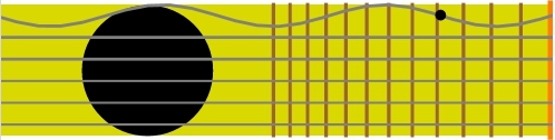
Figure 1:A plucked guitar string is the classic system governed by the 1D wave equation.

Solving the wave equation: the big picture¶

1. Boundary conditions. For a string of length $L$ fixed at both ends, the displacement must vanish at the clamps at all times:

u(0, t) = 0 \quad \text{and} \quad u(L, t) = 0

(2)

2. Separation of variables. We look for solutions in which the dependence on $x$ and on $t$ factorizes, $u(x, t) = X(x) \, T(t)$ . Such a product is a standing wave: a fixed shape $X(x)$ whose overall height $T(t)$ oscillates. This guess turns the PDE into two ordinary differential equations (ODEs), one for each variable.
3. Principle of superposition. The wave equation is linear ( $u$ appears to the first power on both sides), so any linear combination of solutions is a solution. Once we have found all the separable solutions $u_n = X_n(x)T_n(t)$ , the general solution is their sum:

u = \sum_n c_n u_n

(3)

Step 1: Plug the product $X(x)T(t)$ into the wave equation¶

Substitute $u(x, t) = X(x)T(t)$ into the wave equation:

\frac{1}{v^2}\frac{\partial^2 u}{\partial t^2} = \frac{\partial^2 u}{\partial x^2}

(4)

Since $X$ does not depend on $t$ and $T$ does not depend on $x$ , each partial derivative acts on one factor only:

\frac{X(x)}{v^2}\frac{d^2 T}{d t^2} = T(t)\frac{d^2 X}{d x^2}

(5)

Divide both sides by $X(x)T(t)$ :

\frac{1}{v^2\, T(t)}\frac{d^2 T}{d t^2} = \frac{1}{X(x)}\frac{d^2 X}{d x^2}

(6)

The left side depends only on $t$ and the right side only on $x$ . A function of $t$ alone can equal a function of $x$ alone for all $x$ and $t$ only if both are the same constant, which we call $K$ :

\frac{1}{v^2\, T}\frac{d^2 T}{d t^2} = \frac{1}{X}\frac{d^2 X}{d x^2} = K

(7)

One PDE has become two ODEs:

\frac{d^2 X}{d x^2} - K X = 0, \qquad \frac{d^2 T}{d t^2} - K v^2\, T = 0

(8)

Step 2: Solve each ordinary differential equation¶

Solving linear, homogeneous ODEs with constant coefficients

From an ODE to an algebraic equation

An ODE is linear if $y$ and its derivatives appear only to the first power, and homogeneous if the right-hand side is zero. For such equations the trial function $y(x) = e^{rx}$ works, because every derivative of $e^{rx}$ is a multiple of $e^{rx}$ .
Plugging it in and cancelling the common factor $e^{rx}$ leaves an algebraic equation for $r$ , the characteristic equation. For a second-order ODE it is a quadratic:

a y^{''} + by^{'} + cy = 0 \quad \longrightarrow \quad ar^2 + br + c = 0, \qquad r_{1,2} = \frac{-b \pm \sqrt{b^2 - 4ac}}{2a}

(9)

The general solution is a linear combination of the two exponentials. Two extra pieces of information (boundary or initial conditions) fix $c_1$ and $c_2$ :

y(x) = c_1e^{r_1 x}+c_2 e^{r_2 x}

(10)

Example

\frac{d^2 y}{dx^2} +4y = 0 \quad \longrightarrow \quad r^2 + 4 = 0 \quad \longrightarrow \quad r=\pm 2i

(11)

y=c_1e^{2ix} + c_2e^{-2ix} = C_1\cos(2x) + C_2\sin(2x)

(12)

Complex roots $r = \pm i\beta$ always mean oscillation, and Euler’s formula converts the complex exponentials into sines and cosines with new real constants $C_1$ , $C_2$ . Real roots mean exponential growth or decay; a repeated root gives $(c_1 + c_2 x)e^{rx}$ .

The damped oscillator, $y'' + 2\beta y' + \omega^2 y = 0$ , shows what the root type means for the motion. Its characteristic equation has roots $r = -\beta \pm \sqrt{\beta^2 - \omega^2}$ : complex when the damping is weak, real when it is strong. The full solution is worked out in Problem 2 at the end of the chapter.

# synced: damped_oscillator
import numpy as np
import matplotlib.pyplot as plt
from matplotlib.animation import FuncAnimation
from IPython.display import HTML

TEAL, CARDINAL, GRAY, PURPLE, ORANGE = "#107895", "#C8102E", "#6c757d", "#6a3d9a", "#e07b00"
plt.rcParams.update({"axes.spines.top": False, "axes.spines.right": False})
w, b_under, b_over = 2 * np.pi, 0.45, 5.0 * np.pi          # omega, weak and strong damping
t = np.linspace(0, 4, 400)
ts = np.linspace(0, 4, 40)
wd = np.sqrt(w**2 - b_under**2)
y_under = np.exp(-b_under * t) * (np.cos(wd * t) + (b_under / wd) * np.sin(wd * t))
r1, r2 = -b_over + np.sqrt(b_over**2 - w**2), -b_over - np.sqrt(b_over**2 - w**2)
y_over = (r2 * np.exp(r1 * t) - r1 * np.exp(r2 * t)) / (r2 - r1)
y_crit = (1 + w * t) * np.exp(-w * t)
YLO, YHI, TOP = -1.3, 1.95, 1.85                             # shared y range, spring anchor

spring_xy = lambda y_mass, n=9, half=0.16: (                # zigzag from the anchor to the mass
    np.concatenate([[0.0], half * (-1.0) ** np.arange(2 * n), [0.0]]),
    np.linspace(TOP, y_mass + 0.14, 2 * n + 2))

fig = plt.figure(figsize=(8, 3.2))
gs = fig.add_gridspec(1, 4, width_ratios=[1, 3.4, 1, 3.4], wspace=0.32)
ax_s1, ax1, ax_s2, ax2 = [fig.add_subplot(gs[0, i]) for i in range(4)]
for ax_s, fluid, col in ((ax_s1, "water", "#d6ecf5"), (ax_s2, "honey", "#f4d9a4")):
    ax_s.set_xlim(-0.6, 0.6); ax_s.set_ylim(YLO, YHI); ax_s.set_axis_off()
    ax_s.fill_between([-0.6, 0.6], YLO, TOP + 0.02, color=col, zorder=0)
    ax_s.plot([-0.5, 0.5], [TOP, TOP], color="k", lw=3)
    ax_s.axhline(0, color=GRAY, lw=0.8, ls=":")
    ax_s.text(0, YLO + 0.12, fluid, ha="center", fontsize=10.5, color="#444444")
for ax in (ax1, ax2):
    ax.axhline(0, color=GRAY, lw=0.8)
    ax.set_xlim(0, 4); ax.set_ylim(YLO, YHI); ax.set_xlabel("t / T"); ax.set_yticks([-1, 0, 1])
ax1.plot(t, np.exp(-b_under * t), color=GRAY, lw=1, ls="--")
ax1.plot(t, -np.exp(-b_under * t), color=GRAY, lw=1, ls="--")
ax1.text(2.4, 0.5, r"$\pm e^{-\beta t}$", color=GRAY, fontsize=10)
ax1.set_title(r"complex roots $r=-\beta\pm i\omega_d$: oscillates, decays", loc="left", fontsize=10)
ax2.plot(t, y_crit, color=GRAY, lw=1.2, ls="--")
ax2.text(1.1, 0.42, "critical", color=GRAY, fontsize=10)
ax2.set_title(r"real roots $r_1, r_2<0$: no oscillation", loc="left", fontsize=10)
(l1,) = ax1.plot([], [], color=TEAL, lw=2.4)
(d1,) = ax1.plot([], [], "o", color=TEAL, ms=8, mec="white", mew=1.2, zorder=5)
(l2,) = ax2.plot([], [], color=CARDINAL, lw=2.4)
(d2,) = ax2.plot([], [], "o", color=CARDINAL, ms=8, mec="white", mew=1.2, zorder=5)
(sp1,) = ax_s1.plot([], [], color="#444444", lw=1.4)
(m1,) = ax_s1.plot([], [], "s", color=TEAL, ms=15, mec="white", mew=1.2, zorder=5)
(sp2,) = ax_s2.plot([], [], color="#444444", lw=1.4)
(m2,) = ax_s2.plot([], [], "s", color=CARDINAL, ms=15, mec="white", mew=1.2, zorder=5)
fig.subplots_adjust(left=0.02, right=0.985, top=0.88, bottom=0.18)

def update(i):
    n = int(np.searchsorted(t, ts[i])) + 1
    yu, yo = y_under[n - 1], y_over[n - 1]
    l1.set_data(t[:n], y_under[:n]); d1.set_data([t[n - 1]], [yu])
    l2.set_data(t[:n], y_over[:n]); d2.set_data([t[n - 1]], [yo])
    sp1.set_data(*spring_xy(yu)); m1.set_data([0], [yu])
    sp2.set_data(*spring_xy(yo)); m2.set_data([0], [yo])

ani = FuncAnimation(fig, update, frames=len(ts), interval=100, blit=False)
plt.close(fig)
HTML(ani.to_jshtml())

Fig. A mass on a spring released in water (left) and in honey (right). Left: complex roots $r = -\beta \pm i\omega_d$ give an oscillation inside a decaying envelope; the imaginary part sets the frequency, the real part the decay. Right: two real negative roots give decay with no oscillation, the dashed curve being the critically damped case. The spatial equation $X'' - KX = 0$ faces the same fork, decided by the sign of $K$ .

Solving the spatial part when $K > 0$

If $K > 0$ , write $K = \beta^2$ . The characteristic equation $r^2 - \beta^2 = 0$ has real roots $r = \pm\beta$ , so
$X(x) = c_1 e^{\beta x} + c_2 e^{-\beta x}$
(13)
Apply the boundary conditions. $X(0) = 0$ gives $c_2 = -c_1$ , and then $X(L) = c_1\left(e^{\beta L} - e^{-\beta L}\right) = 0$ forces $c_1 = 0$ , because the bracket is not zero for $\beta L \neq 0$ . Only the trivial solution survives:
$X(x) = 0$
(14)
A string that does not move makes no music. Growing and decaying exponentials cannot be pinned to zero at both ends; positive $K$ is ruled out.

Solving the spatial part when $K < 0$

If $K < 0$ , write $K = -\beta^2$ . The characteristic equation $r^2 + \beta^2 = 0$ has imaginary roots $r = \pm i\beta$ :
$X(x) = c_1 e^{i \beta x} + c_2 e^{-i \beta x}$
(15)
Using Euler’s formula, $e^{\pm i\beta x} = \cos(\beta x) \pm i \sin(\beta x)$ , and collecting terms:
$X(x) = (c_1 + c_2) \cos(\beta x) + i(c_1 - c_2) \sin(\beta x) = A \cos(\beta x) + B \sin(\beta x)$
(16)
Apply the boundary conditions:
- At $x = 0$ : $X(0) = A \cdot 1 + B \cdot 0 = 0$ , so $A = 0$ .
- At $x = L$ : $X(L) = B \sin(\beta L) = 0$ .
For a non-trivial solution $B \neq 0$ , so we need $\sin(\beta L) = 0$ . The sine vanishes only at integer multiples of $\pi$ :
$\beta L = n \pi \quad \Longrightarrow \quad \beta_n = \frac{n \pi}{L}, \qquad n = 1, 2, 3, \ldots$
(17)
The boundary conditions have quantized $\beta$ . Every allowed value gives one solution:
$X_n(x) = B_n \sin \left(\frac{n \pi x}{L} \right)$
(18)
The value $n = 0$ gives $X = 0$ and negative $n$ only flips the sign of $B_n$ , so the distinct solutions are $n = 1, 2, 3, \ldots$

# synced: sign_of_k
import numpy as np
import matplotlib.pyplot as plt
from matplotlib.animation import FuncAnimation
from IPython.display import HTML

TEAL, CARDINAL, GRAY, PURPLE, ORANGE = "#107895", "#C8102E", "#6c757d", "#6a3d9a", "#e07b00"
plt.rcParams.update({"axes.spines.top": False, "axes.spines.right": False})
L, b = 1.0, 3.0
x = np.linspace(0, L, 400)
fig, (ax1, ax2) = plt.subplots(1, 2, figsize=(8, 2.0))
for ax in (ax1, ax2):
    ax.axhline(0, color=GRAY, lw=0.8)
    for xc in (0, L):
        ax.plot([xc], [0], "o", color="k", ms=6, zorder=5)
    ax.set_xlim(-0.03, L + 0.03); ax.set_yticks([]); ax.set_xticks([0, L]); ax.set_xticklabels(["0", "L"])
    ax.spines["left"].set_visible(False)
ax1.plot(x, np.exp(b * x) / np.exp(b * L), color=CARDINAL, lw=2.4, label=r"$e^{\beta x}$")
ax1.plot(x, np.exp(-b * x), color=ORANGE, lw=2.4, label=r"$e^{-\beta x}$")
ax1.set_ylim(-0.15, 1.15)
ax1.legend(loc="upper center", fontsize=10, frameon=False, ncol=2)
for n, c in ((1, TEAL), (2, PURPLE)):
    ax2.plot(x, np.sin(n * np.pi * x / L), color=c, lw=2.4, label=r"$\sin(\pi x/L)$" if n == 1 else rf"$\sin({n}\pi x/L)$")
ax2.set_ylim(-1.15, 1.15)
ax2.legend(loc="lower left", fontsize=10, frameon=False)
fig.tight_layout()
plt.show()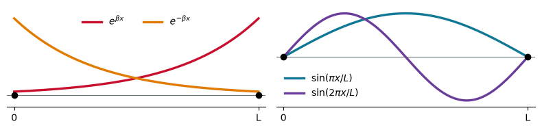

Fig. Why the sign of $K$ decides. Left: for $K > 0$ the solutions are growing and decaying exponentials, and no combination of them returns to zero at both clamps. Right: for $K < 0$ the solutions are sines and cosines, and the sines vanish at both clamps whenever a whole number of half-wavelengths fits.

Solving the temporal part

The spatial part has forced $K = -\beta_n^2$ with $\beta_n = n\pi/L$ . Insert this into the time ODE:

\frac{d^2 T}{d t^2} - K v^2\, T = 0 \quad \Longrightarrow \quad \frac{d^2 T}{d t^2} + \beta_n^2 v^2\, T = 0

(19)

This is the harmonic-oscillator equation with characteristic roots $r = \pm i\beta_n v$ . Its solution oscillates at the angular frequency $\omega_n = \beta_n v$ :

T_n(t) = D_n \cos(\omega_n t) + E_n \sin(\omega_n t), \qquad \omega_n = \beta_n v = \frac{n \pi v}{L}

(20)

Solution for the spatial part: normal modes¶

Because of the boundary conditions $X(0)=X(L)=0$ imposed at the ends of the string, we found an infinite number of solutions indexed by an integer $n$ . These are the normal modes of the string:

The wavelength of the mode follows from $k_n = \beta_n = n\pi/L = 2\pi/\lambda_n$ , so $\lambda_n = 2L/n$ : a whole number of half-wavelengths must fit between the clamps. This is the “waves have to fit” argument of Chapter 1, now derived rather than postulated.

# synced: string_modes
import numpy as np
import matplotlib.pyplot as plt
from matplotlib.animation import FuncAnimation
from IPython.display import HTML

TEAL, CARDINAL, GRAY, PURPLE, ORANGE = "#107895", "#C8102E", "#6c757d", "#6a3d9a", "#e07b00"
plt.rcParams.update({"axes.spines.top": False, "axes.spines.right": False})
L = 1.0
x = np.linspace(0, L, 600)
lam = [r"$\lambda_1 = 2L$", r"$\lambda_2 = L$", r"$\lambda_3 = 2L/3$", r"$\lambda_4 = L/2$"]

fig, axes = plt.subplots(4, 1, figsize=(6.6, 5.6), sharex=True)
for ax, n in zip(axes, range(1, 5)):
    y = np.sin(n * np.pi * x / L)
    ax.plot(x, y, color=TEAL, lw=2.4); ax.plot(x, -y, color=TEAL, lw=1.4, alpha=0.45)
    ax.fill_between(x, y, -y, color=TEAL, alpha=0.08)
    nodes = np.arange(0, n + 1) * L / n
    ax.plot(nodes, np.zeros_like(nodes), "o", color=CARDINAL, ms=7, zorder=5)
    ax.axhline(0, color=GRAY, lw=0.6)
    ax.set_ylim(-1.3, 1.3); ax.set_yticks([]); ax.spines["left"].set_visible(False)
    plural = "s" if n - 1 != 1 else ""
    ax.text(1.03, 0, f"n = {n}\n{n-1} interior node{plural}\n" + lam[n - 1],
            transform=ax.get_yaxis_transform(), va="center", fontsize=10.5)
for ax in axes[:-1]:
    ax.spines["bottom"].set_visible(False); ax.tick_params(axis="x", which="both", bottom=False)
axes[-1].set_xlim(0, L); axes[-1].set_xticks([0, L]); axes[-1].set_xticklabels(["0", "L"]); axes[-1].set_xlabel("x")
fig.suptitle(r"normal modes $X_n(x) = \sin(n\pi x/L)$ of a string fixed at both ends", fontsize=12.5)
fig.tight_layout(rect=(0, 0, 0.8, 0.96))
plt.show()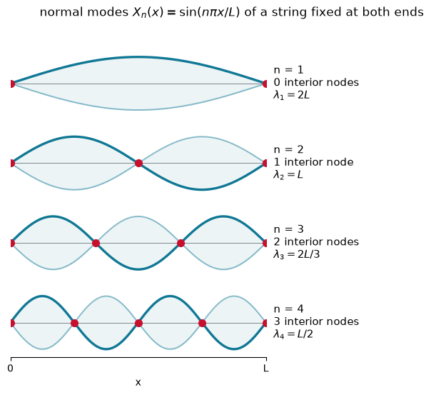

Fig. The first four normal modes at their two extreme positions. Red dots mark the nodes, points that never move; mode $n$ has $n-1$ of them between the clamps and wavelength $2L/n$ .

Solution for the temporal part¶

For the temporal part there are no boundary conditions: time is free to march on. The solution is a linear combination of sine and cosine with $\omega_n = \beta_n v = n \pi v/L$ , which a trig identity packages into a single cosine with an amplitude and a phase:

T_n(t) = D_n \cos(\omega_n t) + E_n \sin(\omega_n t) = A_n \cos (\omega_n t + \phi_n)

(22)

Each mode has its own frequency, and the frequencies are integer multiples of the fundamental $\omega_1 = \pi v/L$ . This is special to the string; a drumhead or an atom does not have equally spaced frequencies.
The constants $A_n$ and $\phi_n$ are not fixed by the equation or by the boundary conditions. They are determined by the initial conditions: where the string is and how fast it is moving at $t=0$ .

Step 3: Full solution as a sum of normal modes¶

Each product $X_n(x)T_n(t)$ is a standing wave that solves the wave equation and respects the clamps. By superposition, so does any sum of them, and the sum over all $n$ is general enough to describe every possible motion of the string:

The normal modes $X_n(x)$ are a property of the string alone (its length and its clamps). How much of each mode is present, the $A_n$ and $\phi_n$ , depends on how and where the string is plucked.

About nodes¶

Places where the string stays at rest are called nodes. Their number grows with $n$ :

$n = 1$ : no interior node. This is the fundamental or first harmonic.
$n = 2$ : one node at $x = L/2$ . The first overtone or second harmonic.
$n = 3$ : two nodes at $L/3$ and $2L/3$ . The second overtone or third harmonic.

A single mode is a standing wave with fixed nodes. A sum of modes is not: because the modes oscillate at different frequencies, the points of zero displacement move around, and the shape changes from instant to instant.

# synced: mode_superposition
import numpy as np
import matplotlib.pyplot as plt
from matplotlib.animation import FuncAnimation
from IPython.display import HTML

TEAL, CARDINAL, GRAY, PURPLE, ORANGE = "#107895", "#C8102E", "#6c757d", "#6a3d9a", "#e07b00"
plt.rcParams.update({"axes.spines.top": False, "axes.spines.right": False})
L, v = 1.0, 1.0
x = np.linspace(0, L, 600)
ts = np.linspace(0, 2 * L / v, 40, endpoint=False)     # one period of the fundamental
X = lambda n: np.sin(n * np.pi * x / L)
Tt = lambda n, t: np.cos(n * np.pi * v * t / L)
combos = [[1], [3], [1, 2], [1, 2, 3]]
titles = ["n = 1", "n = 3", "n = 1 + 2", "n = 1 + 2 + 3"]

fig, axes = plt.subplots(2, 2, figsize=(8, 5.6))
axes = axes.ravel()
lines = []
for ax, ttl in zip(axes, titles):
    (ln,) = ax.plot([], [], color=CARDINAL, lw=2.4); lines.append(ln)
    ax.plot([0, L], [0, 0], "o", color=GRAY, ms=6); ax.axhline(0, color=GRAY, lw=0.6)
    ax.set_xlim(0, L); ax.set_ylim(-2.6, 2.6); ax.set_yticks([])
    ax.set_title(ttl, fontsize=11.5, loc="left")
    ax.set_xticks([0, L]); ax.set_xticklabels(["0", "L"])
fig.suptitle("single modes are standing waves; sums of modes are not", fontsize=12.5)
fig.tight_layout()

def update(i):
    t = ts[i]
    for ln, combo in zip(lines, combos):
        ln.set_data(x, sum(X(n) * Tt(n, t) for n in combo))

ani = FuncAnimation(fig, update, frames=len(ts), interval=90, blit=False)
plt.close(fig)
HTML(ani.to_jshtml())

Fig. Top: single modes $n=1$ and $n=3$ oscillate in place with fixed nodes. Bottom: sums of modes with equal amplitudes; the shape sloshes back and forth because each mode runs at its own frequency.

Initial conditions pick the amplitudes: the plucked string¶

The normal modes are fixed by the string; the amplitudes $A_n$ and phases $\phi_n$ are fixed by how it is set in motion. Suppose the string is pulled into a shape $u(x,0)=f(x)$ and released from rest, so that $\partial u/\partial t = 0$ at $t=0$ . Zero initial velocity kills every $\sin(\omega_n t)$ term, i.e. all $\phi_n = 0$ , and the shape condition reads

f(x) = \sum_{n=1}^\infty A_n \sin\left(\frac{n\pi x}{L}\right)

(24)

To extract a single $A_m$ , multiply both sides by $\sin(m\pi x/L)$ and integrate over the string. The sine modes are orthogonal:

\int_0^L \sin\left(\frac{n\pi x}{L}\right)\sin\left(\frac{m\pi x}{L}\right)dx = \begin{cases} L/2 & n = m \\ 0 & n \neq m \end{cases}

(25)

so every term of the sum vanishes except the one with $n=m$ :

This is a Fourier sine series (Appendix A.6). The move “multiply by a mode and integrate, orthogonality does the rest” is the single most reused calculation in this course: in Chapter 3 it expands a quantum state in eigenfunctions, and the $A_n$ become probability amplitudes.

Example: a string plucked off center

Pull the string at $x=a$ up to height $h$ and let go. The initial shape is a triangle, $f = hx/a$ for $x<a$ and $f=h(L-x)/(L-a)$ for $x>a$ . Integrating by parts (or with SymPy) gives

A_n = \frac{2hL^2}{\pi^2 n^2\, a(L-a)}\sin\left(\frac{n\pi a}{L}\right)

(27)

Two lessons sit in this formula. The amplitudes fall off as $1/n^2$ , so a handful of modes carries most of the motion. And $A_n = 0$ whenever $\sin(n\pi a/L)=0$ : a mode with a node at the pluck point is not excited. Plucking at $a = L/3$ silences $n=3,6,9,\ldots$ ; plucking at the midpoint silences every even harmonic; in the animation below, plucked at $a = 0.3L$ , the tenth harmonic is missing.

# synced: plucked_string
import numpy as np
import matplotlib.pyplot as plt
from matplotlib.animation import FuncAnimation
from IPython.display import HTML

TEAL, CARDINAL, GRAY, PURPLE, ORANGE = "#107895", "#C8102E", "#6c757d", "#6a3d9a", "#e07b00"
plt.rcParams.update({"axes.spines.top": False, "axes.spines.right": False})
L, v, h, a = 1.0, 1.0, 1.0, 0.3            # length, speed, pluck height, pluck position
N = 40                                      # modes kept
n = np.arange(1, N + 1)
A = 2 * h * L**2 * np.sin(n * np.pi * a / L) / (np.pi**2 * n**2 * a * (L - a))
x = np.linspace(0, L, 600)
modes = np.sin(np.outer(n, np.pi * x / L))
omega = n * np.pi * v / L
ts = np.linspace(0, 2 * L / v, 40, endpoint=False)
f0 = np.where(x < a, h * x / a, h * (L - x) / (L - a))

fig, (ax, bx) = plt.subplots(2, 1, figsize=(7.5, 5.8), gridspec_kw={"height_ratios": [1.5, 1]})
ax.plot(x, f0, color=GRAY, lw=1.2, ls=":", label="initial pluck")
(u,) = ax.plot([], [], color=CARDINAL, lw=2.8, label=r"$u(x,t)=\sum_n A_n \sin\frac{n\pi x}{L}\cos\omega_n t$")
(m1,) = ax.plot([], [], color=TEAL, lw=1.4, ls="--", label="n = 1 term")
(m2,) = ax.plot([], [], color=ORANGE, lw=1.4, ls="--", label="n = 2 term")
ax.plot([0, L], [0, 0], "o", color=GRAY, ms=7); ax.axhline(0, color=GRAY, lw=0.6)
ax.set_xlim(-0.02, L + 0.02); ax.set_ylim(-1.15, 1.45); ax.set_yticks([]); ax.set_xlabel("x")
ax.legend(loc="upper right", frameon=False, fontsize=9.5, ncol=2)
ax.set_title("a string plucked at x = 0.3 L, rebuilt from its normal modes", loc="left", fontsize=11.5)
bx.bar(n[:12], A[:12], color=[TEAL if c >= 0 else ORANGE for c in A[:12]], width=0.7)
bx.axhline(0, color=GRAY, lw=0.6)
bx.set_xticks(n[:12]); bx.set_xlabel("mode n"); bx.set_ylabel(r"$A_n$")
bx.set_title(r"the pluck sets the recipe:  $A_n = \frac{2hL^2}{\pi^2 n^2 a(L-a)}\sin\frac{n\pi a}{L}$",
             loc="left", fontsize=11.5)
fig.tight_layout()

def update(i):
    Tn = np.cos(omega * ts[i])
    u.set_data(x, (A * Tn) @ modes)
    m1.set_data(x, A[0] * Tn[0] * modes[0]); m2.set_data(x, A[1] * Tn[1] * modes[1])

ani = FuncAnimation(fig, update, frames=len(ts), interval=90, blit=False)
plt.close(fig)
HTML(ani.to_jshtml())

Fig. Top: a string plucked at $0.3L$ (dotted triangle) evolves as the sum of 40 normal modes (red); the two largest terms are dashed. Bottom: the mode amplitudes $A_n$ . They alternate in sign, fall off as $1/n^2$ , and $A_{10} = 0$ because mode 10 has a node at the pluck point.

The notes of a string¶

Each normal mode oscillates at $\omega_n = n\pi v/L$ , so the frequencies a string can sound are

The fundamental $\nu_1 = v/2L$ sets the pitch. The harmonics (overtones) are its integer multiples, and their mix, the $A_n$ of the previous section, sets the timbre that tells a guitar from a piano playing the same note.

Example: tuning and fretting a guitar

The low E string of a guitar has $L = 0.65\ \text{m}$ and sounds at $\nu_1 = 82.4\ \text{Hz}$ .

A. Wave speed on the string. From $\nu_1 = v/2L$ : $v = 2L\nu_1 = 2(0.65\ \text{m})(82.4\ \text{s}^{-1}) = 107\ \text{m/s}$ .
B. First two overtones. $\nu_2 = 2\nu_1 = 164.8\ \text{Hz}$ and $\nu_3 = 3\nu_1 = 247.2\ \text{Hz}$ .
C. Fretting. Pressing the string at the 12th fret halves its length. With $L \to L/2$ and $v$ unchanged, the fundamental doubles to $164.8\ \text{Hz}$ : one octave up.
D. Tuning. Tightening the string raises $v$ (for a string $v = \sqrt{\mathcal{T}/\mu}$ , tension over mass per unit length), which raises every $\nu_n$ in proportion.

2D membrane vibrations¶

A drumhead is a 2D membrane with fixed edges. Its displacement $u(x, y, t)$ depends on two spatial variables, and separation of variables now uses a product of three functions:

u(x, y, t) = X(x)\, Y(y)\, T(t)

(29)

The boundary conditions on a rectangular membrane of sides $a$ and $b$ pin each spatial factor at its two edges: $X(0) = X(a) = 0$ and $Y(0) = Y(b) = 0$ . Each factor is therefore a 1D normal mode, and the 2D mode is their product, labeled by two integers $n$ and $m$ :

u(x, y, t) = \sum_n \sum_m A_{nm} \cos(\omega_{nm}t + \phi_{nm}) \sin\left(\frac{n\pi x}{a}\right) \sin\left(\frac{m\pi y}{b}\right)

(30)

The frequency of a mode depends on both integers and on the geometry:

Unlike the string, the frequencies are not integer multiples of the lowest one. This is why a drum has no definite pitch while a string does.

# synced: membrane_modes
import numpy as np
import matplotlib.pyplot as plt
from matplotlib.animation import FuncAnimation
from IPython.display import HTML

TEAL, CARDINAL, GRAY, PURPLE, ORANGE = "#107895", "#C8102E", "#6c757d", "#6a3d9a", "#e07b00"
a = b = 1.0
g = np.linspace(0, 1, 41)
X, Y = np.meshgrid(g, g)
pairs = [(1, 1), (2, 1), (1, 2), (2, 2)]
shapes = [np.sin(n * np.pi * X / a) * np.sin(m * np.pi * Y / b) for n, m in pairs]
ts = np.linspace(0, 1, 24, endpoint=False)             # one common period

fig = plt.figure(figsize=(8.4, 6.4))
axes = [fig.add_subplot(2, 2, i + 1, projection="3d") for i in range(4)]
for ax, (n, m) in zip(axes, pairs):
    ratio = np.sqrt((n / a)**2 + (m / b)**2) / np.sqrt(2)
    ax.set_title(rf"(n, m) = ({n}, {m}),   $\omega_{{nm}}/\omega_{{11}}$ = {ratio:.2f}", fontsize=11, pad=0)
    ax.set_zlim(-1, 1); ax.view_init(elev=32, azim=-55); ax.set_box_aspect((1, 1, 0.5), zoom=1.35); ax.set_axis_off()
fig.suptitle("normal modes of a square membrane; (2,1) and (1,2) share one frequency", fontsize=12.5, y=0.98)
fig.subplots_adjust(left=0.0, right=1.0, bottom=0.0, top=0.9, wspace=0.0, hspace=0.05)
surfs = []

def update(i):
    for s in surfs:
        s.remove()
    surfs.clear()
    c = np.cos(2 * np.pi * ts[i])
    for ax, Z in zip(axes, shapes):
        surfs.append(ax.plot_surface(X, Y, c * Z, cmap="RdBu_r", vmin=-1, vmax=1,
                                     rstride=1, cstride=1, linewidth=0, antialiased=True))

ani = FuncAnimation(fig, update, frames=len(ts), interval=110, blit=False)
plt.close(fig)
HTML(ani.to_jshtml())

Fig. The four lowest normal modes of a square membrane, all shown at a common phase so that the shapes can be compared. Each is a product of a sine in $x$ and a sine in $y$ ; the nodal lines where the membrane stays flat are the 2D counterpart of the nodes on a string.

Use the sliders to choose the two mode numbers and rotate the surface.

Full derivation of the 2D rectangular membrane problem

Consider a rectangular membrane with dimensions $L_x$ and $L_y$ , fixed along its edges. The wave equation for the membrane is

\frac{\partial^2 u}{\partial t^2} = v^2 \left( \frac{\partial^2 u}{\partial x^2} + \frac{\partial^2 u}{\partial y^2} \right)

(32)

Separation of variables. Assume $u(x, y, t) = X(x) Y(y) T(t)$ , substitute, and divide through by $X Y T$ :

\frac{1}{v^2} \frac{1}{T} \frac{d^2 T}{dt^2} = \frac{1}{X} \frac{d^2 X}{dx^2} + \frac{1}{Y} \frac{d^2 Y}{dy^2}

(33)

The left side depends only on $t$ , the right side only on $x$ and $y$ , so both equal a constant, which we call $-\lambda$ . On the right, the $x$ term and the $y$ term must in turn each be constant, $-\alpha^2$ and $-\beta^2$ , with $\alpha^2 + \beta^2 = \lambda$ . This gives three ODEs:

\frac{d^2 X}{dx^2} + \alpha^2 X = 0, \qquad \frac{d^2 Y}{dy^2} + \beta^2 Y = 0, \qquad \frac{d^2 T}{dt^2} + \lambda v^2 T = 0

(34)

Boundary conditions. $X(0) = X(L_x) = 0$ and $Y(0) = Y(L_y) = 0$ quantize $\alpha$ and $\beta$ exactly as for the string:

X_n(x) = \sin\left(\frac{n \pi x}{L_x}\right), \quad \alpha_n = \frac{n\pi}{L_x}, \qquad Y_m(y) = \sin\left(\frac{m \pi y}{L_y}\right), \quad \beta_m = \frac{m\pi}{L_y}

(35)

Time part. With $\lambda_{nm} = \alpha_n^2 + \beta_m^2$ , $T$ oscillates at $\omega_{nm} = v\sqrt{\lambda_{nm}}$ .

General solution.

u(x, y, t) = \sum_{n=1}^\infty \sum_{m=1}^\infty \left[ A_{nm} \cos\left(\omega_{nm} t\right) + B_{nm} \sin\left(\omega_{nm} t\right) \right] \sin\left(\frac{n \pi x}{L_x}\right) \sin\left(\frac{m \pi y}{L_y}\right), \qquad \omega_{nm} = v \pi\sqrt{\frac{n^2}{L_x^2} + \frac{m^2}{L_y^2}}

(36)

The sound of music¶

The sound of a musical instrument is a superposition of its normal modes (the harmonics or overtones of music). Which modes are present, and how strongly, depends on how the instrument is excited: where a string is plucked, where a drum is struck.
Learn more from this series.

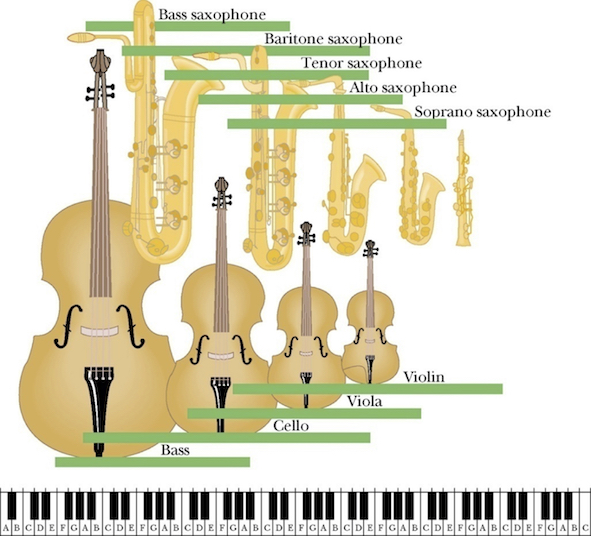
The size of a musical instrument reflects the range of frequencies it is designed to produce: \nu_1 = v/2L, so smaller instruments produce higher frequencies and larger instruments lower ones. — Figure 2:The size of a musical instrument reflects the range of frequencies it is designed to produce: $\nu_1 = v/2L$ , so smaller instruments produce higher frequencies and larger instruments lower ones.

Looking ahead: the same recipe for the Schrödinger equation¶

Everything in this lecture transfers to quantum mechanics with a change of cast. Keep this table in mind when Chapter 3 solves the particle in a box.

classical string	quantum particle in a box
wave equation $u_{xx} = u_{tt}/v^2$	Schrödinger equation $-\frac{\hbar^2}{2m}\Psi_{xx} + V\Psi = i\hbar\Psi_t$
separation $u = X(x)\,T(t)$	separation $\Psi = \psi(x)\,e^{-iEt/\hbar}$
fixed ends $X(0)=X(L)=0$	impenetrable walls $\psi(0)=\psi(L)=0$
normal modes $\sin(n\pi x/L)$	stationary states $\sin(n\pi x/L)$
frequencies $\omega_n \propto n$	energies $E_n \propto n^2$
pluck sets the amplitudes $A_n$	initial state sets the probability amplitudes $c_n$
orthogonality extracts $A_n$	orthogonality extracts $c_n$

The only structural difference is the single time derivative and the factor $i$ in the Schrödinger equation, which is why quantum “oscillation” in time is a rotating complex phase rather than a real cosine.

Problems¶

Problem 1: Simple harmonic oscillator¶

Solve the ODE

\frac{d^2 y}{dt^2} + \omega^2 y = 0

(37)

where $\omega$ is a constant.

Solution

The characteristic equation is

r^2 + \omega^2 = 0 \quad \Longrightarrow \quad r = \pm i \omega

(38)

Thus the general solution is

y(t) = C_1 \cos(\omega t) + C_2 \sin(\omega t)

(39)

where $C_1$ and $C_2$ are constants determined by initial conditions.

Problem 2: Damped oscillator¶

Solve the ODE

\frac{d^2 y}{dt^2} + 2 \beta \frac{dy}{dt} + \omega^2 y = 0

(40)

where $\beta$ and $\omega$ are constants. Consider the cases $\beta^2 < \omega^2$ , $\beta^2 > \omega^2$ , and $\beta^2 = \omega^2$ .

Solution

The characteristic equation is

r^2 + 2 \beta r + \omega^2 = 0 \quad \Longrightarrow \quad r = -\beta \pm \sqrt{\beta^2 - \omega^2}

(41)

Depending on the sign of the discriminant $\beta^2 - \omega^2$ there are three cases:

Underdamping ( $\beta^2 < \omega^2$ ): the roots are complex, $r = -\beta \pm i\omega_d$ with $\omega_d = \sqrt{\omega^2 - \beta^2}$ , giving a decaying oscillation
$y(t) = e^{-\beta t} [C_1 \cos(\omega_d t) + C_2 \sin(\omega_d t)]$
(42)
Critical damping ( $\beta^2 = \omega^2$ ): a repeated root $r = -\beta$ ,
$y(t) = (C_1 + C_2 t) e^{-\beta t}$
(43)
Overdamping ( $\beta^2 > \omega^2$ ): two distinct real (negative) roots $r_1, r_2$ ,
$y(t) = C_1 e^{r_1 t} + C_2 e^{r_2 t}$
(44)

Problem 3: Real roots¶

Solve the ODE

\frac{d^2 y}{dt^2} - 4 y = 0

(45)

Solution

The characteristic equation is $r^2 - 4 = 0$ , so $r = \pm 2$ and

y(t) = C_1 e^{2t} + C_2 e^{-2t}

(46)

Real roots give exponentials, not oscillations. Compare with Problem 4, where the sign of the constant term is flipped.

Problem 4: Imaginary roots¶

Solve the ODE

\frac{d^2 y}{dt^2} + 9 y = 0

(47)

Solution

The characteristic equation is $r^2 + 9 = 0$ , so $r = \pm 3i$ and

y(t) = C_1 \cos(3t) + C_2 \sin(3t)

(48)

Problem 5: Repeated roots¶

Solve the ODE

\frac{d^2 y}{dt^2} - 6 \frac{dy}{dt} + 9 y = 0

(49)

Solution

The characteristic equation factors as $(r - 3)^2 = 0$ , a repeated root $r = 3$ . The general solution for repeated roots is

y(t) = (C_1 + C_2 t) e^{3t}

(50)

Problem 6: A string with one free end¶

A string of length $L$ is clamped at $x=0$ but its other end slides freely on a frictionless rod, so that the slope vanishes there: $X(0) = 0$ and $X'(L) = 0$ . Find the allowed normal modes and their frequencies. Which harmonics of the fixed-fixed string are missing? (A clarinet, closed at one end and open at the other, has the same pattern.)

Problem 7: Plucking at the midpoint¶

A string is pulled to height $h$ at its midpoint and released from rest. Using the formula for $A_n$ in the plucked-string example, compute $A_1$ through $A_5$ in units of $h$ . Which modes are absent, and why can you predict that from the symmetry of the initial shape without any integration?

Problem 8: Frequencies of a square drum¶

For a square membrane of side $a$ , list $\omega_{nm}/\omega_{11}$ for all $n, m \leq 3$ in increasing order. Which frequencies are degenerate? Now make the membrane rectangular with $b = 1.2a$ : which degeneracies survive?

Problem 9: Waves on a ring¶

A wave travels on a closed loop of circumference $L$ , so instead of fixed ends the solution must satisfy periodic boundary conditions, $X(0) = X(L)$ and $X'(0) = X'(L)$ . Show that $X(x) = e^{ikx}$ works when $k = 2\pi n/L$ with $n = 0, \pm 1, \pm 2, \ldots$ , find the wavelengths, and compare with the standing-wave condition on a Bohr orbit in Chapter 1.

Problem 10: Orthogonality of the modes¶

Show by direct integration that

\int_0^L \sin\left(\frac{n\pi x}{L}\right)\sin\left(\frac{m\pi x}{L}\right)dx = \frac{L}{2}\,\delta_{nm}

(51)

for positive integers $n, m$ . (Use $\sin\alpha\sin\beta = \tfrac{1}{2}[\cos(\alpha-\beta)-\cos(\alpha+\beta)]$ .) Then use the result to verify the formula $A_n = \frac{2}{L}\int_0^L f(x)\sin(n\pi x/L)\,dx$ .

Classical wave equation¶

Solving the wave equation: the big picture¶

Step 1: Plug the product X(x)T(t)X(x)T(t)X(x)T(t) into the wave equation¶

Step 2: Solve each ordinary differential equation¶

Solution for the spatial part: normal modes¶

Solution for the temporal part¶

Step 3: Full solution as a sum of normal modes¶

About nodes¶

Initial conditions pick the amplitudes: the plucked string¶

The notes of a string¶

2D membrane vibrations¶

The sound of music¶

Looking ahead: the same recipe for the Schrödinger equation¶

Problems¶

Problem 1: Simple harmonic oscillator¶

Problem 2: Damped oscillator¶

Problem 3: Real roots¶

Problem 4: Imaginary roots¶

Problem 5: Repeated roots¶

Problem 6: A string with one free end¶

Problem 7: Plucking at the midpoint¶

Problem 8: Frequencies of a square drum¶

Problem 9: Waves on a ring¶

Problem 10: Orthogonality of the modes¶

Step 1: Plug the product $X(x)T(t)$ into the wave equation¶