The Schrödinger Equation and the Wavefunction - Quantum Mechanics for Chemistry

What you need to know

Feeding the de Broglie and Planck relations into a complex traveling wave, and demanding that energy is conserved, produces Schrödinger’s equation, the equation of motion of the quantum world.
Separation of variables splits it into a rotating phase $e^{-iEt/\hbar}$ and the time-independent Schrödinger equation for the shape $\psi(x)$ . These product solutions are stationary states: the phase turns, the probability density does not move.
The time-independent equation is a curvature equation. Where $E > V$ the wavefunction oscillates, where $E < V$ it decays or grows. Demanding that it stays finite allows only special energies: quantization comes from boundary conditions, as it did for the string.
The wavefunction is complex and not directly measurable. Its absolute square $|\psi(x)|^2$ is the probability density for finding the particle, so physical wavefunctions must be normalized.
Every measurable quantity corresponds to an operator. Predictions are expectation values $\langle A \rangle = \int \psi^{*} \hat{A}\, \psi\, dx$ , and solving the Schrödinger equation means finding the eigenfunctions $\psi_n$ and eigenvalues $E_n$ of the Hamiltonian.

Why a new equation?¶

Classical mechanics works at large scales and fails for atoms and molecules. Chapter 1 collected the evidence, and any new equation of motion has to build in two facts from it:
- Energy comes in quanta. Blackbody radiation, the photoelectric effect and atomic spectra all require $E = h\nu$ .
- Matter is a wave. Electron diffraction and the double slit show that a particle with momentum $p$ carries a wavelength $\lambda = h/p$ .
Chapter 2 gave us the language of waves: complex exponentials, the wave equation, separation of variables, normal modes. In 1926 Erwin Schrödinger, an expert on the physics of waves, put the two quantum relations into that language and found the equation that the matter wave obeys.
The Schrödinger equation is a fundamental law. It cannot be derived from anything more basic; it can only be motivated and then tested. In the century since, it has passed every test it was given, from the spectrum of hydrogen to the structure of molecules and solids.

A person stepping through a door into a space filled with crossing lines — Figure 1:Fig. Entering the quantum world.

Building the equation¶

We follow Schrödinger’s reasoning in three steps: write down the wave of a free particle, see what its derivatives give back, and then demand that energy is conserved.

Step 1: the wave of a free particle¶

The complex traveling wave of Chapter 2 moves to the right with wavenumber $k = 2\pi/\lambda$ and angular frequency $\omega = 2\pi\nu$ :

\Psi(x,t) = A\,e^{i(kx-\omega t)}

(1)

Now insert the two quantum relations. De Broglie ties the wavenumber to the momentum, and Planck ties the frequency to the energy:

p = \frac{h}{\lambda} = \hbar k, \qquad E = h\nu = \hbar\omega

(2)

The wave has to be complex, and the reason is physical. A free particle with a definite momentum has no preferred position, so the chance of finding it must be the same everywhere and at all times. A real wave $\cos(kx-\omega t)$ cannot do that: its square vanishes at nodes that sweep along with the wave. The complex wave can. Its real and imaginary parts run a quarter cycle apart, so when one is zero the other is at its maximum, and $|\Psi|^2 = \mathrm{Re}^2 + \mathrm{Im}^2$ stays perfectly flat.

# synced: complex_plane_wave
import numpy as np
import matplotlib.pyplot as plt
from matplotlib.animation import FuncAnimation
from IPython.display import HTML

TEAL, CARDINAL, GRAY, PURPLE, ORANGE = "#107895", "#C8102E", "#6c757d", "#6a3d9a", "#e07b00"
plt.rcParams.update({"axes.spines.top": False, "axes.spines.right": False})
k, w = 2 * np.pi / 4.0, 2 * np.pi            # lambda = 4, one period per loop
x = np.linspace(0, 12, 600)
ts = np.linspace(0, 1, 36, endpoint=False)

fig, (ax1, ax2) = plt.subplots(2, 1, figsize=(8, 4.0), sharex=True,
                               gridspec_kw={"height_ratios": [1.25, 1]})
(re,) = ax1.plot([], [], color=TEAL, lw=2.4, label=r"Re $\Psi = \cos(kx-\omega t)$")
(im,) = ax1.plot([], [], color=ORANGE, lw=2.0, ls="--", label=r"Im $\Psi = \sin(kx-\omega t)$")
ax1.axhline(0, color=GRAY, lw=0.6)
ax1.set_ylim(-1.3, 1.95); ax1.set_yticks([-1, 0, 1]); ax1.set_ylabel(r"$\Psi$")
ax1.legend(loc="upper right", frameon=False, fontsize=9.5, ncol=2)
ax1.set_title(r"free particle $\Psi = e^{i(kx-\omega t)}$: two real waves, a quarter cycle apart",
              loc="left", fontsize=11)

real2 = ax2.fill_between(x, 0 * x, color=GRAY, alpha=0.25, lw=0)
(real2_line,) = ax2.plot([], [], color=GRAY, lw=1.4, label=r"a real wave, $\cos^2(kx-\omega t)$: moving dead spots")
ax2.plot(x, np.ones_like(x), color=CARDINAL, lw=2.8, label=r"$|\Psi|^2 = \mathrm{Re}^2 + \mathrm{Im}^2 = 1$ everywhere")
ax2.set_xlim(0, 12); ax2.set_ylim(0, 1.75); ax2.set_yticks([0, 1])
ax2.set_xlabel("x"); ax2.set_ylabel("probability density")
ax2.legend(loc="upper right", frameon=False, fontsize=9.5, ncol=1)
fig.tight_layout()

def update(i):
    ph = k * x - w * ts[i]
    re.set_data(x, np.cos(ph)); im.set_data(x, np.sin(ph))
    real2_line.set_data(x, np.cos(ph) ** 2)
    real2.set_data(x, 0 * x, np.cos(ph) ** 2)

ani = FuncAnimation(fig, update, frames=len(ts), interval=85, blit=False)
plt.close(fig)
HTML(ani.to_jshtml())

Fig. A free particle moving to the right. Top: the real and imaginary parts of $\Psi$ are two ordinary traveling waves a quarter cycle apart. Bottom: their squares add up to a constant, so the particle is equally likely to be found anywhere, while the square of a single real wave would have dead spots moving along $x$ .

Step 2: derivatives pull out the energy and the momentum¶

Differentiate the free-particle wave with respect to time. The exponential comes back multiplied by $-iE/\hbar$ . Moving the constants to the left side:

i\hbar\,\frac{\partial \Psi}{\partial t} = E\,\Psi

(4)

Differentiate with respect to position. One derivative returns the momentum, two derivatives return the kinetic energy:

-i\hbar\,\frac{\partial \Psi}{\partial x} = p\,\Psi, \qquad\qquad -\frac{\hbar^2}{2m}\frac{\partial^2 \Psi}{\partial x^2} = \frac{p^2}{2m}\,\Psi

(5)

Read these three lines as questions put to the wave. The operation $i\hbar\,\partial/\partial t$ asks “what is your energy?”, $-i\hbar\,\partial/\partial x$ asks “what is your momentum?”, and the wave answers by returning itself times the number. This is the first appearance of operators, to which we return at the end of the lecture.

Step 3: demand that energy is conserved¶

A particle moving in a potential $V$ has total energy equal to kinetic plus potential energy:

E = \frac{p^2}{2m} + V

(6)

Multiply both sides by $\Psi$ , then replace $E\Psi$ and $\frac{p^2}{2m}\Psi$ with the derivatives from Step 2:

E\,\Psi = \frac{p^2}{2m}\,\Psi + V\,\Psi \qquad\Longrightarrow\qquad i\hbar\,\frac{\partial \Psi}{\partial t} = -\frac{\hbar^2}{2m}\frac{\partial^2 \Psi}{\partial x^2} + V\,\Psi

(7)

Every term of the equation is an energy acting on the wavefunction, so the equation is energy conservation written in the language of waves:

\underbrace{-\frac{\hbar^2}{2m} \frac{\partial^2 \Psi}{\partial x^2}}_{\substack{\text{kinetic energy:} \\ \text{curvature of } \Psi \text{ in space}}} \;+\; \underbrace{V(x)\,\Psi\vphantom{\frac{\partial^2}{\partial x^2}}}_{\substack{\text{potential energy:} \\ \text{defines the system}}} \;=\; \underbrace{i \hbar \frac{\partial \Psi}{\partial t}\vphantom{\frac{\partial^2}{\partial x^2}}}_{\substack{\text{total energy:} \\ \text{rate of change of } \Psi \text{ in time}}}

(9)

What we did is a motivation and not a derivation. The steps hold for one plane wave and a constant $V$ . Schrödinger’s postulate is that the same equation governs any wavefunction in any potential $V(x)$ . Only the agreement with experiment justifies that leap.
We work in one dimension for simplicity. In three dimensions the second derivative becomes the Laplacian, $\partial^2/\partial x^2 \to \nabla^2$ , and $V$ depends on $x, y, z$ .

Why not reuse the classical wave equation?

The classical wave equation has two derivatives in space and two in time. Acting on $e^{i(kx-\omega t)}$ they bring down $k^2$ and $\omega^2$ , so the equation enforces $\omega = vk$ : frequency proportional to wavenumber.

A free quantum particle obeys a different rule. With $E = \hbar\omega$ and $p = \hbar k$ , the energy $E = p^2/2m$ reads

\omega = \frac{\hbar k^2}{2m}

(10)

so the frequency goes as the square of the wavenumber. An equation that produces one power of $\omega$ and two powers of $k$ needs one time derivative and two space derivatives. The single time derivative returns $-i\omega$ , which is imaginary, while the two space derivatives return $-k^2$ , which is real. The factor $i$ in the Schrödinger equation is there to balance the two sides.

Quantum versus classical wave equation¶

	classical wave equation	Schrödinger equation
equation	$\dfrac{\partial^2 u}{\partial x^2} = \dfrac{1}{v^2}\dfrac{\partial^2 u}{\partial t^2}$	$-\dfrac{\hbar^2}{2m}\dfrac{\partial^2 \Psi}{\partial x^2} + V\Psi = i\hbar\dfrac{\partial \Psi}{\partial t}$
time derivative	second	first, with a factor $i$
the wave	real displacement $u$ , directly measurable	complex $\Psi$ , only $\lvert\Psi\rvert^2$ is measurable
frequency and wavenumber	$\omega = vk$	$\omega = \hbar k^2/2m$ for a free particle
what defines the system	wave speed $v$ and the boundaries	mass $m$ , potential $V(x)$ and the boundaries
time dependence of a mode	real oscillation $\cos(\omega_n t)$	rotating phase $e^{-iE_n t/\hbar}$
linear, so solutions add	yes	yes

Solving the equation: separation of variables¶

The equation is linear and, as long as $V$ does not depend on time, it separates. The recipe is the one we used for the vibrating string.

Step 1: plug in a product¶

Look for solutions in which the dependence on $x$ and on $t$ factorizes, $\Psi(x,t) = \psi(x)\,T(t)$ . Each derivative acts on one factor only:

i\hbar\,\psi(x)\,\frac{dT}{dt} = T(t)\left[-\frac{\hbar^2}{2m}\frac{d^2\psi}{dx^2} + V(x)\,\psi\right]

(11)

Divide both sides by $\psi(x)T(t)$ :

i\hbar\,\frac{1}{T}\frac{dT}{dt} = \frac{1}{\psi}\left[-\frac{\hbar^2}{2m}\frac{d^2\psi}{dx^2} + V(x)\,\psi\right]

(12)

The left side depends only on $t$ and the right side only on $x$ , so both must equal the same constant. It has units of energy, and we call it $E$ . One PDE has become two ODEs.

Step 2: the time part is a rotating phase¶

The time equation is first order, $dT/dt = -(iE/\hbar)\,T$ . The trial function $e^{rt}$ gives a single root $r = -iE/\hbar$ , which is purely imaginary. In Chapter 2 imaginary roots meant oscillation, and the same holds here:

T(t) = e^{-iEt/\hbar}

(13)

This is a point moving around the unit circle of the complex plane with angular frequency $\omega = E/\hbar$ . The separation constant is the energy of Planck’s relation $E = \hbar\omega$ , which justifies its name.

Step 3: the spatial part is the time-independent Schrödinger equation¶

Almost all of the work in this course goes into this equation. The potential $V(x)$ defines the system, and solving the equation gives the shapes $\psi(x)$ and the energies $E$ the system can have.

Stationary states: the phase turns, the density stays¶

The name comes from the probability density. The time factor has absolute value one, so it drops out:

|\Psi(x,t)|^2 = |\psi(x)|^2\,\left|e^{-iEt/\hbar}\right|^2 = |\psi(x)|^2

(16)

The real and imaginary parts of $\Psi$ slosh back and forth forever, yet nothing measurable moves. A string mode of Chapter 2 passes through the flat shape twice per period. A stationary state never goes flat, because its imaginary part is at its largest when its real part vanishes.
The animation uses the two lowest states of a particle held between two walls. Their shapes are the sines of the string modes, as we will show in the next lecture. The second state has four times the energy, so its phase clock runs four times faster.

# synced: phase_clock
import numpy as np
import matplotlib.pyplot as plt
from matplotlib.animation import FuncAnimation
from IPython.display import HTML

TEAL, CARDINAL, GRAY, PURPLE, ORANGE = "#107895", "#C8102E", "#6c757d", "#6a3d9a", "#e07b00"
plt.rcParams.update({"axes.spines.top": False, "axes.spines.right": False})
x = np.linspace(0, 1, 300)
ts = np.linspace(0, 1, 36, endpoint=False)    # one full turn of the n = 1 clock
th = np.linspace(0, 2 * np.pi, 200)
fig = plt.figure(figsize=(8, 4.3))
gs = fig.add_gridspec(2, 2, width_ratios=[3.4, 1], hspace=0.5, wspace=0.08)
rows = []
for r, n in enumerate((1, 2)):
    ax, axc = fig.add_subplot(gs[r, 0]), fig.add_subplot(gs[r, 1])
    psi = np.sqrt(2) * np.sin(n * np.pi * x)
    ax.fill_between(x, psi**2, color=CARDINAL, alpha=0.12, lw=0)
    ax.plot(x, psi**2, color=CARDINAL, lw=1.8, label=r"$|\Psi|^2$ (does not move)")
    (re,) = ax.plot([], [], color=TEAL, lw=2.4, label=r"Re $\Psi$")
    (im,) = ax.plot([], [], color=ORANGE, lw=2.0, ls="--", label=r"Im $\Psi$")
    ax.axhline(0, color=GRAY, lw=0.6)
    ax.set_xlim(0, 1); ax.set_ylim(-1.7, 2.3); ax.set_yticks([-1, 0, 1, 2])
    ax.set_xticks([0, 0.5, 1]); ax.set_xticklabels(["0", "L/2", "L"])
    ax.set_title(rf"$\Psi_{n}(x,t) = \psi_{n}(x)\,e^{{-iE_{n}t/\hbar}}$" + ("" if n == 1 else r",  $E_2 = 4E_1$"),
                 loc="left", fontsize=11)
    if r == 0:
        ax.legend(loc="upper right", frameon=False, fontsize=9, ncol=3, bbox_to_anchor=(1.0, 1.32))
    axc.plot(np.cos(th), np.sin(th), color=GRAY, lw=1, ls="--")
    axc.axhline(0, color=GRAY, lw=0.6); axc.axvline(0, color=GRAY, lw=0.6)
    (hand,) = axc.plot([], [], color=PURPLE, lw=2.8)
    (tip,) = axc.plot([], [], "o", color=PURPLE, ms=7)
    axc.set_aspect("equal"); axc.set_xlim(-1.25, 1.25); axc.set_ylim(-1.25, 1.25); axc.set_axis_off()
    axc.set_title("phase clock" if r == 0 else "4 times faster", fontsize=10, color=PURPLE)
    rows.append((n, psi, re, im, hand, tip))
fig.subplots_adjust(left=0.06, right=0.99, top=0.86, bottom=0.08)

def update(i):
    for n, psi, re, im, hand, tip in rows:
        z = np.exp(-2j * np.pi * n**2 * ts[i])
        re.set_data(x, psi * z.real); im.set_data(x, psi * z.imag)
        hand.set_data([0, z.real], [0, z.imag]); tip.set_data([z.real], [z.imag])

ani = FuncAnimation(fig, update, frames=len(ts), interval=110, blit=False)
plt.close(fig)
HTML(ani.to_jshtml())

Fig. Two stationary states of a particle between walls at 0 and $L$ . The real and imaginary parts oscillate at the rate $E_n/\hbar$ set by the phase clock on the right, while the probability density $|\Psi|^2$ stays fixed.

The time-independent equation is a curvature equation¶

Solve the time-independent equation for the second derivative:

\frac{d^2\psi}{dx^2} = -\frac{2m}{\hbar^2}\,\big[E - V(x)\big]\,\psi

(17)

This is the spatial equation of the string, $X'' = KX$ , with $K = -\frac{2m}{\hbar^2}(E - V)$ . There the sign of $K$ decided between sines and exponentials. Here the sign of $E - V(x)$ decides, and it can change from place to place:
- Allowed region, $E > V$ . The kinetic energy $E - V$ is positive. The curvature has the opposite sign to $\psi$ , so the wavefunction always bends back toward the axis and oscillates. The larger $E - V$ , the stronger the curvature and the shorter the wavelength, in line with de Broglie: $\lambda = h/\sqrt{2m(E-V)}$ .
- Forbidden region, $E < V$ . A classical particle could never be here, since its kinetic energy would be negative. The curvature has the same sign as $\psi$ , so the wavefunction bends away from the axis: it decays or grows exponentially. It is not zero there, a fact that leads to tunneling.

# synced: allowed_forbidden
import numpy as np
import matplotlib.pyplot as plt
from matplotlib.animation import FuncAnimation
from IPython.display import HTML

TEAL, CARDINAL, GRAY, PURPLE, ORANGE = "#107895", "#C8102E", "#6c757d", "#6a3d9a", "#e07b00"
plt.rcParams.update({"axes.spines.top": False, "axes.spines.right": False})
a, V0, N = 1.2, 30.0, 700                     # half width, depth (units hbar^2/2m = 1)
x = np.linspace(-3.4, 3.4, N); h = x[1] - x[0]
V = np.where(np.abs(x) < a, 0.0, V0)
H = (np.diag(2.0 / h**2 + V) - np.diag(np.ones(N - 1) / h**2, 1)
     - np.diag(np.ones(N - 1) / h**2, -1))
En, vec = np.linalg.eigh(H)
n = 3                                         # fourth level: three nodes, long tails
E, psi = En[n], vec[:, n] / np.abs(vec[:, n]).max()
psi = psi * np.sign(psi[np.argmax(np.abs(psi))])

fig, ax = plt.subplots(figsize=(8, 3.4))
ax.axvspan(-a, a, color=TEAL, alpha=0.08, lw=0)
ax.axvspan(-3.4, -a, color=CARDINAL, alpha=0.06, lw=0)
ax.axvspan(a, 3.4, color=CARDINAL, alpha=0.06, lw=0)
ax.plot(x, V, color="k", lw=2.0)
ax.axhline(E, color=GRAY, lw=1.2, ls="--")
ax.plot(x, E + 7.5 * psi, color=TEAL, lw=2.6)
ax.text(3.35, E + 0.9, "E", color=GRAY, fontsize=11, ha="right")
ax.text(3.35, V0 + 0.9, "V(x)", color="k", fontsize=11, ha="right")
ax.text(0, 38.5, r"allowed, $E > V$" + "\n" + r"$\psi$ curves toward the axis: oscillates",
        ha="center", va="top", fontsize=10, color=TEAL)
for xc in (-2.35, 2.35):
    ax.text(xc, 38.5, r"forbidden, $E < V$" + "\n" + "curves away: decays",
            ha="center", va="top", fontsize=10, color=CARDINAL)
ax.set_xlim(-3.4, 3.4); ax.set_ylim(-2, 39.5)
ax.set_xlabel("x"); ax.set_ylabel("energy"); ax.set_yticks([])
fig.tight_layout()
plt.show()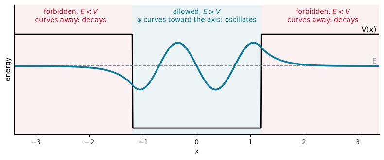

Fig. The fourth state of a particle in a well of finite depth, drawn on its energy level. Inside the well $E > V$ and $\psi$ oscillates; in the walls $E < V$ and $\psi$ decays.

Why only some energies are allowed¶

In a forbidden region the general solution is a mix of a decaying and a growing exponential. A wavefunction that grows without limit cannot describe a particle, so the growing part has to be absent on the left and on the right.
For most energies this is impossible. Start the solution so that it decays properly on the left and follow the curvature equation across the well: it arrives on the right side with some of the growing exponential mixed in, and it blows up. Only at special energies does the solution arrive with the right slope to decay on both sides. These are the allowed energies.
Try it for a particle on a spring, $V = \frac{1}{2}kx^2$ . The cell below starts from a tiny value on the far left and integrates the curvature equation to the right for the trial energy you choose. Find the energies between 0 and $3\,\hbar\omega$ for which the right tail comes down to the axis, and count the nodes of each solution.

Fig. A trial solution of the time-independent equation for a particle on a spring, drawn on its energy level. It is bounded only at $E = \frac{1}{2}, \frac{3}{2}, \frac{5}{2}$ in units of $\hbar\omega$ .

The pattern is the one we met on the string, where clamped ends allowed only the wavelengths that fit. Here the requirement that $\psi$ stays finite allows only the energies that fit. The Schrödinger equation does not contain quantization; the boundary conditions put it there. Each new allowed state has one more node than the one below it.
The allowed energies of the spring turn out to be evenly spaced, $E_n = (n + \frac{1}{2})\hbar\omega$ . We derive this in Chapter 4, where it explains molecular vibrations.

What does the wavefunction mean?¶

We now have the equation and a strategy for solving it. What we do not have yet is the meaning of the object the equation keeps handing us.

In the classical wave equation, $u(x,t)$ is something you can see: the height of a guitar string above its resting position. The quantum wavefunction is complex, so it cannot stand for any measurable quantity by itself.
The interpretation that survived every experimental test was proposed by Max Born in 1926. The wavefunction is a probability amplitude, and its absolute square is a probability density:

One measurement of position gives one dot at one place, and the wavefunction does not say where the next dot lands. Its content shows up only in the statistics: repeat the experiment on many identically prepared particles, and the dots pile up in proportion to $|\psi(x)|^2$ . Where $\psi$ has a node, no particle is ever found.

# synced: born_buildup
import numpy as np
import matplotlib.pyplot as plt
from matplotlib.animation import FuncAnimation
from IPython.display import HTML

TEAL, CARDINAL, GRAY, PURPLE, ORANGE = "#107895", "#C8102E", "#6c757d", "#6a3d9a", "#e07b00"
plt.rcParams.update({"axes.spines.top": False, "axes.spines.right": False})
rng = np.random.default_rng(7)
cand = rng.random(14000)
hits = cand[rng.random(14000) < np.sin(2 * np.pi * cand) ** 2][:3000]   # samples of 2 sin^2(2 pi x)
yj = rng.random(3000)
counts = np.unique(np.round(np.geomspace(1, 3000, 40)).astype(int))
edges = np.linspace(0, 1, 31); mid = 0.5 * (edges[1:] + edges[:-1]); dx = edges[1] - edges[0]
xs = np.linspace(0, 1, 300)

fig, (ax_s, ax_h) = plt.subplots(2, 1, figsize=(8, 4.0), sharex=True,
                                 gridspec_kw={"height_ratios": [1, 2.3]})
scat = ax_s.scatter([], [], s=5, color=TEAL, alpha=0.6, lw=0)
ax_s.set_ylim(0, 1); ax_s.set_yticks([])
for sp in ("left", "bottom"):
    ax_s.spines[sp].set_visible(False)
ax_s.tick_params(bottom=False)
bars = ax_h.bar(mid, np.zeros_like(mid), width=0.92 * dx, color=TEAL, alpha=0.5, label="detections per bin")
(curve,) = ax_h.plot([], [], color=CARDINAL, lw=2.6, label=r"prediction $N\,|\psi(x)|^2\,\Delta x$")
ax_h.set_xlim(0, 1); ax_h.set_yticks([])
ax_h.set_xticks([0, 0.5, 1]); ax_h.set_xticklabels(["0", "L/2", "L"])
ax_h.set_xlabel("position x"); ax_h.set_ylabel("detections")
ax_h.legend(loc="upper center", frameon=False, fontsize=9.5, ncol=2, bbox_to_anchor=(0.5, 1.17))
ax_s.set_title("N = 1 detection, one dot each", loc="left", fontsize=11)
fig.tight_layout()

def update(i):
    N = counts[i]
    scat.set_offsets(np.column_stack([hits[:N], yj[:N]]))
    hist = np.histogram(hits[:N], bins=edges)[0]
    for b, c in zip(bars, hist):
        b.set_height(c)
    curve.set_data(xs, N * dx * 2 * np.sin(2 * np.pi * xs) ** 2)
    ax_h.set_ylim(0, 1.3 * max(1.0, hist.max(), 2 * N * dx))
    ax_s.set_title(f"N = {N} detection" + ("" if N == 1 else "s") + ", one dot each", loc="left", fontsize=11)

ani = FuncAnimation(fig, update, frames=len(counts), interval=160, blit=False)
plt.close(fig)
HTML(ani.to_jshtml())

Fig. Position measurements on particles that were all prepared in the same state $\psi_2$ . Single detections look random; the histogram of many detections converges to $|\psi_2(x)|^2$ , with a gap at the node.

The same holds in three dimensions, where $|\psi(x,y,z)|^2\,dx\,dy\,dz$ is the probability of finding the particle in a small volume. The “electron cloud” pictures of chemistry are this statement: each dot below is one position measurement on a hydrogen atom in its ground state, and the cloud of many dots traces out the 1s orbital.

# synced: h1s_cloud
import numpy as np
import matplotlib.pyplot as plt
from matplotlib.animation import FuncAnimation
from IPython.display import HTML

TEAL, CARDINAL, GRAY, PURPLE, ORANGE = "#107895", "#C8102E", "#6c757d", "#6a3d9a", "#e07b00"
plt.rcParams.update({"axes.spines.top": False, "axes.spines.right": False})
rng = np.random.default_rng(11)
N = 5000
r = 0.5 * rng.gamma(shape=3.0, scale=1.0, size=N)       # P(r) = 4 r^2 exp(-2r), r in units of a0
cos_t = 1 - 2 * rng.random(N); phi = 2 * np.pi * rng.random(N)
xx, zz = r * np.sqrt(1 - cos_t**2) * np.cos(phi), r * cos_t
rr = np.linspace(0, 6, 300)

fig, (ax1, ax2) = plt.subplots(1, 2, figsize=(8, 3.5), gridspec_kw={"width_ratios": [1, 1.35]})
ax1.scatter(xx, zz, s=2, color=TEAL, alpha=0.45, lw=0)
ax1.plot([0], [0], "+", color=CARDINAL, ms=9, mew=1.8)
ax1.set_aspect("equal"); ax1.set_xlim(-5, 5); ax1.set_ylim(-5, 5)
ax1.set_xlabel(r"x / $a_0$"); ax1.set_ylabel(r"z / $a_0$")
ax1.set_title(f"{N} position measurements", loc="left", fontsize=11)
ax2.hist(r, bins=np.linspace(0, 6, 49), density=True, color=TEAL, alpha=0.45, label="measured distances")
ax2.plot(rr, 4 * rr**2 * np.exp(-2 * rr), color=CARDINAL, lw=2.6, label=r"$4\pi r^2\,|\psi_{1s}|^2$")
ax2.set_xlim(0, 6); ax2.set_xlabel(r"distance from the nucleus r / $a_0$"); ax2.set_ylabel("probability density")
ax2.legend(frameon=False, fontsize=10)
ax2.set_title("the dots follow the wavefunction", loc="left", fontsize=11)
fig.tight_layout()
plt.show()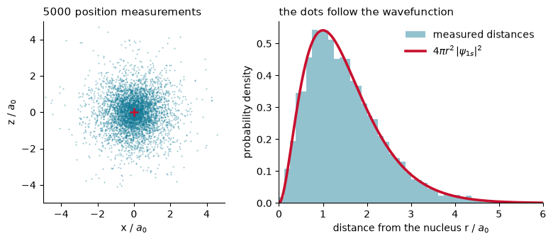

Fig. Left: simulated position measurements of the electron in the hydrogen 1s state, projected on a plane. Right: the measured distances from the nucleus follow the radial distribution computed from the wavefunction (Chapter 5).

Probability refresher

A random variable assigns a number to the outcome of an experiment. It can be discrete (a die roll, a coin flip) or continuous (the position of a particle). A continuous random variable is described by a probability density $p(x)$ with these properties:

Non-negative: $p(x) \geq 0$ .
Normalized: $\int_{-\infty}^{\infty} p(x)\,dx = 1$ , because the outcome is certain to lie somewhere.
Mean: $\langle x \rangle = \int x\,p(x)\,dx$ , and for any function $\langle f \rangle = \int f(x)\,p(x)\,dx$ .
Variance: $\sigma^2 = \langle x^2 \rangle - \langle x \rangle^2$ , the squared width of the distribution.

For a discrete variable the integrals become sums, $\langle x \rangle = \sum_i x_i\,p_i$ .

Fair coin, $X \in \{0, 1\}$ with $p_0 = p_1 = \frac{1}{2}$ : the mean is $\langle X\rangle = 0\cdot\frac{1}{2} + 1\cdot\frac{1}{2} = \frac{1}{2}$ , and since $\langle X^2\rangle = \frac{1}{2}$ the variance is $\sigma^2 = \frac{1}{2} - \frac{1}{4} = \frac{1}{4}$ .

Uniform density on $[0,1]$ , $p(x) = 1$ : the mean is $\int_0^1 x\,dx = \frac{1}{2}$ , the mean square is $\int_0^1 x^2dx = \frac{1}{3}$ , and $\sigma^2 = \frac{1}{3} - \frac{1}{4} = \frac{1}{12}$ .

Gaussian, $p(x) = \frac{1}{\sqrt{2\pi}\,\sigma}e^{-(x-\mu)^2/2\sigma^2}$ : normalized, with mean $\mu$ and variance $\sigma^2$ .

More practice: a video overview and an interactive probability explorer.

Normalization¶

The particle is certain to be found somewhere, so the probabilities must add up to one:

The Schrödinger equation is linear, so if $\psi'$ solves it then $N\psi'$ does too, for any constant $N$ . The equation therefore never fixes the overall size of a wavefunction. Normalization does: substitute $\psi = N\psi'$ into the condition and solve for $N$ .
A wavefunction that cannot be normalized, because the integral of $|\psi'|^2$ is infinite, does not describe a particle. This is the requirement that ruled out the diverging solutions in the slider above.
In three dimensions the integral runs over all of space, $\iiint |\psi(x,y,z)|^2\,dx\,dy\,dz = 1$ .

# synced: normalization_area
import numpy as np
import matplotlib.pyplot as plt
from matplotlib.animation import FuncAnimation
from IPython.display import HTML

TEAL, CARDINAL, GRAY, PURPLE, ORANGE = "#107895", "#C8102E", "#6c757d", "#6a3d9a", "#e07b00"
plt.rcParams.update({"axes.spines.top": False, "axes.spines.right": False})
x = np.linspace(0, 1, 300)
fig, (ax1, ax2) = plt.subplots(1, 2, figsize=(8, 2.9), sharey=True)
for ax, c, col, lab, area in ((ax1, 1.0, GRAY, r"$\psi' = x$", "area = 1/3"),
                              (ax2, 3.0, TEAL, r"$\psi = \sqrt{3}\,x$", "area = 1")):
    ax.fill_between(x, c * x**2, color=col, alpha=0.25, lw=0)
    ax.plot(x, c * x**2, color=col, lw=2.6)
    ax.text(0.06, 2.55, lab, fontsize=12, color=col)
    ax.text(0.80, 0.18 * c + 0.05, area, fontsize=11, ha="center", color="k")
    ax.set_xlim(0, 1); ax.set_ylim(0, 3.1); ax.set_xlabel("x")
ax1.set_ylabel(r"$|\psi(x)|^2$")
ax1.set_title("not normalized", loc="left", fontsize=11)
ax2.set_title("normalized: a probability density", loc="left", fontsize=11)
fig.tight_layout()
plt.show()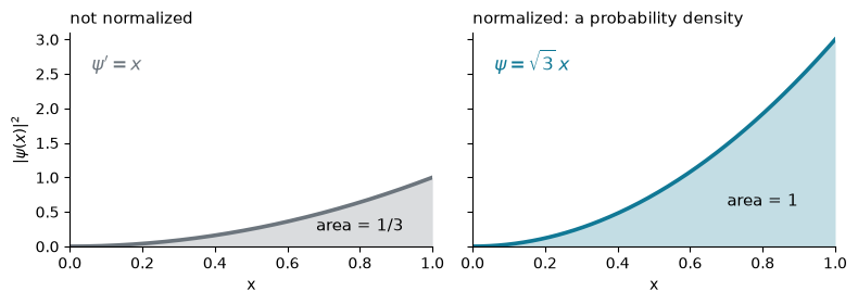

Fig. Normalization rescales the wavefunction until the area under $|\psi|^2$ equals one.

Probability of finding the particle in a region¶

Once $\psi$ is normalized, the probability of finding the particle anywhere between $a$ and $b$ is the area under $|\psi|^2$ over that interval:

In three dimensions the same integral runs over a volume.

Move the edges of the region and check the example.

Fig. The probability of finding the particle in a region is the shaded area under $|\psi|^2$ .

Mean and spread of position¶

A probability density also predicts averages. The mean of many position measurements is the expectation value of $x$ , and the spread of the results around it is the standard deviation $\sigma_x$ :

$\langle x \rangle$ is the balance point of the density. It is not the most likely position, and it need not even be a position where the particle can be found: for $\psi_2$ in the animation above, $\langle x \rangle = L/2$ sits exactly on the node.

# synced: mean_and_spread
import numpy as np
import matplotlib.pyplot as plt
from matplotlib.animation import FuncAnimation
from IPython.display import HTML

TEAL, CARDINAL, GRAY, PURPLE, ORANGE = "#107895", "#C8102E", "#6c757d", "#6a3d9a", "#e07b00"
plt.rcParams.update({"axes.spines.top": False, "axes.spines.right": False})
x = np.linspace(0, 1, 2001)
fig, axes = plt.subplots(1, 2, figsize=(8, 3.0), sharey=True)
for ax, p, col, lab in ((axes[0], 3 * x**2, TEAL, r"$|\psi|^2 = 3x^2$"),
                        (axes[1], 2 * np.sin(np.pi * x) ** 2, ORANGE, r"$|\psi_1|^2 = 2\sin^2(\pi x)$")):
    mu = np.trapezoid(x * p, x)
    sig = np.sqrt(np.trapezoid(x**2 * p, x) - mu**2)
    ax.fill_between(x, p, color=col, alpha=0.2, lw=0); ax.plot(x, p, color=col, lw=2.6)
    ax.axvspan(mu - sig, mu + sig, color=PURPLE, alpha=0.12, lw=0)
    ax.axvline(mu, color=PURPLE, lw=1.6)
    ax.plot([mu], [-0.16], marker="^", color=PURPLE, ms=11, clip_on=False, zorder=6)
    ax.set_title(lab + rf":  $\langle x\rangle = {mu:.2f}$,  $\sigma_x = {sig:.2f}$", loc="left", fontsize=10.5)
    ax.set_xlim(0, 1); ax.set_ylim(0, 3.2); ax.set_xlabel("x")
    ax.set_xticks([0, 0.25, 0.5, 0.75, 1]); ax.tick_params(axis="x", pad=9)
axes[0].set_ylabel("probability density")
axes[0].text(0.75 - 0.21, 2.75, r"$\pm\sigma_x$", color=PURPLE, fontsize=11, ha="right")
fig.tight_layout()
plt.show()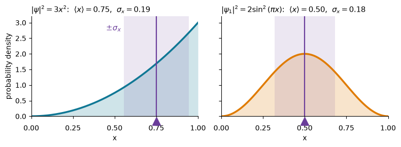

Fig. The mean (line and triangle) is the balance point of the probability density, and the band marks one standard deviation on each side. Left: the density of the example. Right: the ground state of a particle between walls, whose mean sits at the center by symmetry.

Operators: a first look¶

Position was easy, because $x$ is just a number that multiplies $|\psi|^2$ . Momentum and energy are different. In Step 2 we extracted them from the wave by differentiating, and that idea organizes the rest of quantum mechanics. This section is a preview; Operators 1, Operators 2 and Eigenvalues and Expectation Values develop it in full.

An operator is an instruction that turns one function into another, written with a hat. Every observable of classical mechanics has a quantum operator. The recipe: write the classical expression in terms of $x$ and $p$ , then replace $p$ with $-i\hbar\,\partial/\partial x$ .

observable	classical	quantum operator
position	$x$	$\hat{x} = x$
momentum	$p = mv$	$\hat{p} = -i\hbar \dfrac{\partial}{\partial x}$
potential energy	$V(x)$	$\hat{V} = V(x)$
kinetic energy	$K = \dfrac{p^2}{2m}$	$\hat{K} = \dfrac{\hat{p}^2}{2m} = -\dfrac{\hbar^2}{2m}\dfrac{\partial^2}{\partial x^2}$
total energy	$H = \dfrac{p^2}{2m} + V(x)$	$\hat{H} = \hat{K} + \hat{V}$

The operator of the total energy is the Hamiltonian, named after the total energy function $H(x,p)$ of classical mechanics. With it both Schrödinger equations fit on one line.

Different systems differ only in $V(x)$ : $V = 0$ is a free particle, $V = \frac{1}{2}kx^2$ a particle on a spring (a vibrating bond), $V = -e^2/4\pi\epsilon_0 r$ the electron of a hydrogen atom.

Eigenfunctions and eigenvalues¶

An operator usually changes the shape of the function it acts on. The special functions that come back unchanged, multiplied by a constant, are its eigenfunctions, and the constant is the eigenvalue:

\hat{A} f(x) = a\, f(x)

(28)

# synced: eigen_test
import numpy as np
import matplotlib.pyplot as plt
from matplotlib.animation import FuncAnimation
from IPython.display import HTML

TEAL, CARDINAL, GRAY, PURPLE, ORANGE = "#107895", "#C8102E", "#6c757d", "#6a3d9a", "#e07b00"
plt.rcParams.update({"axes.spines.top": False, "axes.spines.right": False})
x = np.linspace(-3, 3, 500); a = 1.5
fig, (ax1, ax2) = plt.subplots(1, 2, figsize=(8, 3.0))
ax1.plot(x, np.sin(a * x), color=TEAL, lw=2.6, label=r"$f = \sin(ax)$")
ax1.plot(x, -a**2 * np.sin(a * x), color=CARDINAL, lw=2.2, ls="--", label=r"$f'' = -a^2 \sin(ax)$")
ax1.set_title(r"same shape, rescaled: eigenfunction of $d^2/dx^2$", loc="left", fontsize=10.5)
ax2.plot(x, np.exp(-x**2), color=TEAL, lw=2.6, label=r"$f = e^{-x^2}$")
ax2.plot(x, (4 * x**2 - 2) * np.exp(-x**2), color=CARDINAL, lw=2.2, ls="--", label=r"$f'' = (4x^2-2)\,e^{-x^2}$")
ax2.set_title("new shape: not an eigenfunction", loc="left", fontsize=10.5)
for ax in (ax1, ax2):
    ax.axhline(0, color=GRAY, lw=0.6); ax.set_xlim(-3, 3); ax.set_ylim(-2.6, 3.6); ax.set_xlabel("x")
    ax.legend(loc="upper right", frameon=False, fontsize=9.5)
fig.tight_layout()
plt.show()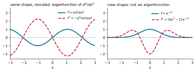

Fig. Testing two functions against the operator $d^2/dx^2$ . Left: $\sin(ax)$ comes back with the same shape, multiplied by $-a^2$ , so it is an eigenfunction. Right: the Gaussian comes back with a different shape, so it is not.

The time-independent Schrödinger equation is exactly such a problem. The slider above was a search for its eigenvalues by hand.

Expectation values¶

For position we averaged $x$ over the density $\psi^*\psi$ . An operator such as $\hat{p}$ has to act on $\psi$ before we multiply by $\psi^*$ , so it sits between the two:

average	operator inside the integral
$\langle x \rangle=\int \psi^{*}\, x\, \psi\, dx$	$\hat{x} = x$
$\langle p \rangle=\int \psi^{*}\, \hat{p}\, \psi\, dx$	$\hat{p}=-i\hbar\dfrac{d}{dx}$
$\langle K \rangle=\int \psi^{*}\, \hat{K}\, \psi\, dx$	$\hat{K}=-\dfrac{\hbar^2}{2m}\dfrac{d^2}{dx^2}$
$\langle E \rangle=\int \psi^{*}\, \hat{H}\, \psi\, dx$	$\hat{H}=-\dfrac{\hbar^2}{2m}\dfrac{d^2}{dx^2}+V(x)$

Example: momentum and energy of a particle between walls

Take $\psi_n(x)=\sqrt{2}\sin(n\pi x)$ on $[0,1]$ with $V = 0$ inside.

Momentum. The derivative turns the sine into a cosine, and $\sin\cos = \frac{1}{2}\sin(2n\pi x)$ integrates to zero over the box:

\langle p\rangle = \int_0^1 \psi_n\,(-i\hbar)\,\frac{d\psi_n}{dx}\,dx = -2i\hbar\, n\pi \int_0^1 \sin(n\pi x)\cos(n\pi x)\,dx = 0

(31)

The particle is as likely to move left as right.

Momentum squared and energy. Two derivatives return the sine, $\psi_n'' = -(n\pi)^2\psi_n$ , so

\langle p^2\rangle = -\hbar^2\int_0^1 \psi_n\,\psi_n''\,dx = (n\pi\hbar)^2, \qquad \langle E\rangle = \frac{\langle p^2\rangle}{2m} = \frac{(n\pi\hbar)^2}{2m}

(32)

The average momentum vanishes but the average of its square does not: the particle is moving, with no preferred direction.

Linearity and superposition¶

$\hat{H}$ is a linear operator, so any sum of solutions is again a solution. As for the string, the general solution is a sum over the stationary states, each turning at its own rate:

\Psi(x,t) = \sum_n c_n\, \psi_n(x)\, e^{-iE_n t/\hbar}

(33)

A single stationary state has a frozen probability density. A sum of two does not, because their phase clocks run at different rates and the relative phase changes in time (Problem 2). All motion in quantum mechanics comes from superposition, the subject of Time Dependence.

Looking ahead¶

The next lecture carries out this program for the simplest potential there is: a particle in a box, $V = 0$ between two impenetrable walls. The curvature equation gives sines, the walls pick out the allowed ones, normalization fixes their height, and the expectation values of this lecture turn them into predictions.

Problems¶

Problem 1: The plane wave solves the free equation¶

Show that $\Psi(x,t) = A\,e^{\frac{i}{\hbar}(px - Et)}$ solves the time-dependent Schrödinger equation with $V = 0$ only if $E = p^2/2m$ .

Solution

Two derivatives in $x$ bring down $(ip/\hbar)^2 = -p^2/\hbar^2$ , so the left side is

-\frac{\hbar^2}{2m}\frac{\partial^2\Psi}{\partial x^2} = \frac{p^2}{2m}\,\Psi

(34)

One derivative in $t$ brings down $-iE/\hbar$ , so the right side is

i\hbar\frac{\partial \Psi}{\partial t} = i\hbar\left(-\frac{iE}{\hbar}\right)\Psi = E\,\Psi

(35)

The two sides agree for all $x$ and $t$ only if $E = p^2/2m$ . The equation accepts a plane wave of any momentum, but it ties the frequency to the wavenumber: $\omega = \hbar k^2/2m$ .

Problem 2: One stationary state stands still, two do not¶

Let $\psi_1$ and $\psi_2$ be real, normalized stationary states with energies $E_1$ and $E_2$ . Compute the probability density $|\Psi|^2$ of the superposition

\Psi(x,t) = \frac{1}{\sqrt{2}}\left[\psi_1(x)\,e^{-iE_1t/\hbar} + \psi_2(x)\,e^{-iE_2t/\hbar}\right]

(36)

and find the frequency at which it oscillates.

Solution

Multiply $\Psi$ by its complex conjugate. The two squared terms lose their phases; the two cross terms keep the difference of the phases:

|\Psi|^2 = \frac{1}{2}\left[\psi_1^2 + \psi_2^2 + \psi_1\psi_2\left(e^{i(E_2-E_1)t/\hbar} + e^{-i(E_2-E_1)t/\hbar}\right)\right]

(37)

|\Psi|^2 = \frac{1}{2}\left[\psi_1^2 + \psi_2^2\right] + \psi_1\psi_2\cos\left(\frac{(E_2-E_1)\,t}{\hbar}\right)

(38)

The density sloshes at the angular frequency $\omega_{21} = (E_2 - E_1)/\hbar$ . Only energy differences appear, which is the Bohr frequency condition $h\nu = E_2 - E_1$ of atomic spectra.

Problem 3: Normalize and locate¶

Normalize $\psi(x) = N\cos(\pi x / 2)$ on the interval $[-1, 1]$ , then compute the probability of finding the particle in $[0, \tfrac{1}{2}]$ .

Solution

Use $\cos^2\theta = \frac{1}{2}(1 + \cos 2\theta)$ :

\int_{-1}^{1} N^2\cos^2\left(\frac{\pi x}{2}\right)dx = \frac{N^2}{2}\int_{-1}^{1}\left[1 + \cos(\pi x)\right]dx = \frac{N^2}{2}\left[2 + 0\right] = N^2

(39)

so $N = 1$ : the function was already normalized. The probability is

P\left(0 < x < \tfrac{1}{2}\right) = \frac{1}{2}\int_0^{1/2}\left[1 + \cos(\pi x)\right]dx = \frac{1}{2}\left[\frac{1}{2} + \frac{1}{\pi}\right] \approx 0.41

(40)

A quarter of the interval holds 41 percent of the probability, because the density peaks at the center.

Problem 4: Eigenfunctions of momentum and kinetic energy¶

Decide whether each function is an eigenfunction of the momentum operator, of the kinetic energy operator, of both, or of neither:

$A \sin(ax)$
$N e^{-ikx}$

Solution

Apply the momentum operator to the first function:

-i \hbar \dfrac{\partial}{\partial x} A \sin(ax) = -i \hbar A a \cos(ax)

(41)

The sine turned into a cosine, so $\sin(ax)$ is not an eigenfunction of momentum. The kinetic energy operator gives

-\dfrac{\hbar^2}{2m} \dfrac{\partial^2}{\partial x^2} A \sin(ax) = \dfrac{\hbar^2 a^2}{2m}\, A \sin(ax)

(42)

The same function came back, so $\sin(ax)$ is an eigenfunction of kinetic energy with eigenvalue $\hbar^2a^2/2m$ .

For the second function:

-i\hbar \dfrac{\partial}{\partial x} N e^{-ikx} = -i\hbar(-ik)\,N e^{-ikx} = -\hbar k\, N e^{-ikx}

(43)

It is an eigenfunction of momentum with eigenvalue $-\hbar k$ : a wave moving to the left. Applying the momentum operator twice gives $\hat{K} N e^{-ikx} = \frac{\hbar^2k^2}{2m} N e^{-ikx}$ , so it is an eigenfunction of kinetic energy too.

A state of definite momentum always has a definite kinetic energy. The reverse is not true: $\sin(ax)$ is an equal mix of $e^{iax}$ and $e^{-iax}$ , waves moving right and left with the same kinetic energy.

Problem 5: Testing a Gaussian¶

Check whether $f(x) = e^{-\alpha x^2}$ is an eigenfunction of $\hat{C} = \dfrac{d^2}{dx^2}$ .

Solution

\frac{d}{dx} e^{-\alpha x^2} = -2\alpha x\, e^{-\alpha x^2}

(44)

\frac{d^2}{dx^2} e^{-\alpha x^2} = \left( 4\alpha^2 x^2 - 2\alpha \right) e^{-\alpha x^2}

(45)

The factor in front depends on $x$ , so the result is not a constant times $f$ : the Gaussian is not an eigenfunction of $d^2/dx^2$ . This is the right panel of the eigenfunction figure, with $\alpha = 1$ . Notice, though, that $\left(-\frac{d^2}{dx^2} + 4\alpha^2x^2\right)f = 2\alpha f$ : the Gaussian is an eigenfunction once a potential proportional to $x^2$ is added. It is the ground state of the particle on a spring that you found with the slider.

Problem 6: Find the levels by hand¶

Use the trial-energy slider to find every allowed energy of the particle on a spring below $3\,\hbar\omega$ . For each one record the number of nodes. How is the number of nodes related to the order of the levels? Compare with the modes of a string.

Problem 7: Allowed and forbidden regions¶

A particle with energy $E$ moves in $V(x) = \frac{1}{2}kx^2$ . Find the two turning points where $E = V$ . Sketch the state with two nodes and mark where $\psi$ oscillates and where it decays. Where is the local wavelength shortest, and why?

Problem 8: A particle in a cube¶

Let $\psi(x,y,z)=\sqrt{27}\,xyz$ inside the unit cube $[0,1]^3$ and zero outside. Verify that $\psi$ is normalized, then find the probability that the particle is in the corner box $[0,\frac{1}{2}]^3$ . Compare with the fraction of the volume that the box takes up.

Problem 9: Symmetry does the integrals¶

For the state $\psi_2(x) = \sqrt{2}\sin(2\pi x)$ on $[0, 1]$ , evaluate $\langle x \rangle$ and $\langle p \rangle$ , and explain both results using symmetry alone.

Problem 10: Spread of the ground state¶

For $\psi_1(x) = \sqrt{2}\sin(\pi x)$ on $[0,1]$ compute $\langle x^2 \rangle$ and $\sigma_x$ , and compare with the value quoted in the figure on mean and spread. (Integrate by parts, or use $\sin^2\theta = \frac{1}{2}(1-\cos 2\theta)$ .)