Waves - Quantum Mechanics for Chemistry

What you will learn

A wave is a self-propagating disturbance that carries energy, momentum, and information through a medium without transporting matter. We describe it by a function of position and time, $u(x,t)$ .
Any shape that moves without changing form is a function of $x \mp vt$ . The periodic case is the sine wave $A\sin(kx-\omega t)$ , and its complex form $Ae^{i(kx-\omega t)}$ turns the algebra of waves into multiplication.
Two periodicities: the wavelength $\lambda$ in space and the period $T$ in time, packaged as $k=2\pi/\lambda$ and $\omega=2\pi/T$ and tied together by the speed, $v=\omega/k=\lambda\nu$ .
Every wave $f(x \mp vt)$ obeys the same equation, the classical wave equation $u_{xx}=u_{tt}/v^2$ .
Waves add. Because the wave equation is linear, interference, standing waves, and beats are all superpositions of simpler waves.
Light is the one wave without a medium. Its speed is the same for every observer, and that single fact forces moving clocks to run slow.

Types of waves¶

Disturbance of a medium: sound waves, waves on a guitar string, ripples on the surface of water.
Quantum mechanical waves: described by complex wavefunctions, which explain the wave-like behavior of electrons and atoms.
Electromagnetic waves (light, UV, X-rays): the only kind of wave that needs no medium. EM waves travel in vacuum; in a sense an EM wave “rolls out its own carpet,” creating its own medium as it moves forward.
Gravitational waves traveling through spacetime.

Waves also differ in which way the medium moves. In a transverse wave the disturbance is perpendicular to the direction of travel (a string, light). In a longitudinal wave the disturbance is along the direction of travel (sound in air, a compressed spring). In both cases the beads of the medium only oscillate about their resting positions; only the pattern travels.

# synced: transverse_longitudinal
import numpy as np
import matplotlib.pyplot as plt
from matplotlib.animation import FuncAnimation
from IPython.display import HTML

TEAL, CARDINAL, GRAY, PURPLE, ORANGE = "#107895", "#C8102E", "#6c757d", "#6a3d9a", "#e07b00"
plt.rcParams.update({"axes.spines.top": False, "axes.spines.right": False})
N, A, k, w = 48, 0.35, 2 * np.pi / 4.0, 2 * np.pi / 2.0   # beads, amplitude, lambda = 4, T = 2
x0 = np.linspace(0, 12, N)
xs = np.linspace(0, 12, 600)
ts = np.linspace(0, 2 * np.pi / w, 40, endpoint=False)
pick = 18                                                 # the bead we follow

fig, (ax1, ax2) = plt.subplots(2, 1, figsize=(8, 4.6))
for ax in (ax1, ax2):
    ax.set_xlim(-0.5, 12.5); ax.set_ylim(-1.3, 1.45)
    ax.set_yticks([]); ax.spines["left"].set_visible(False)
    ax.annotate("", xy=(12.3, 1.1), xytext=(10.3, 1.1), arrowprops=dict(arrowstyle="->", color=GRAY, lw=1.6))
    ax.text(11.3, 1.22, "wave moves", color=GRAY, fontsize=10, ha="center")
    ax.axvline(x0[pick], color=CARDINAL, lw=1, ls=":")
ax1.set_title("transverse: each bead moves up and down, perpendicular to the wave", loc="left", fontsize=11.5)
ax2.set_title("longitudinal: each bead moves back and forth, along the wave", loc="left", fontsize=11.5)
ax2.set_xlabel("x")
(string,) = ax1.plot([], [], color=TEAL, lw=1.2, alpha=0.6)
(beads1,) = ax1.plot([], [], "o", color=TEAL, ms=5)
(red1,) = ax1.plot([], [], "o", color=CARDINAL, ms=9, mec="white", mew=1.2, zorder=5)
(beads2,) = ax2.plot([], [], "o", color=TEAL, ms=6)
(red2,) = ax2.plot([], [], "o", color=CARDINAL, ms=9, mec="white", mew=1.2, zorder=5)
fig.tight_layout()

def update(i):
    t = ts[i]
    string.set_data(xs, 0.8 * np.sin(k * xs - w * t))
    beads1.set_data(x0, 0.8 * np.sin(k * x0 - w * t))
    red1.set_data([x0[pick]], [0.8 * np.sin(k * x0[pick] - w * t)])
    xl = x0 + A * np.sin(k * x0 - w * t)
    beads2.set_data(xl, np.zeros(N))
    red2.set_data([xl[pick]], [0])

ani = FuncAnimation(fig, update, frames=len(ts), interval=75, blit=False)
plt.close(fig)
HTML(ani.to_jshtml())

Fig. Transverse and longitudinal waves on a line of beads. The red bead never travels with the wave; it oscillates about the dotted line while the pattern moves to the right. In the longitudinal case the wave shows up as traveling regions of compression and rarefaction.

Defining a wave mathematically¶

Since a wave is a moving disturbance $u$ , we describe this disturbance (e.g. the vertical displacement of a string) as a function of space $x$ and time $t$ :

u = f(x, t)

(1)

Imagine surfing on an ocean wave. For an observer riding the wave, the wave stays still at the same coordinate $x'$ .
For an observer standing on the shore, the coordinate $x$ of the wave front moves away with a constant velocity:

x=x'+vt

(2)

Assuming that the shape of the wave stays the same, the shore observer sees the surfer’s frozen shape $f(x')$ carried along:

u(x,t) = f(x')=f(x-vt)

(3)

To see why $f(x-vt)$ moves to the right, follow one point of the shape, say its peak, by holding the argument fixed: $x-vt=\text{const}$ gives $x = vt +\text{const}$ , a point moving right at speed $v$ . The same reasoning shows that $f(x+vt)$ moves to the left.

# synced: traveling_pulse
import numpy as np
import matplotlib.pyplot as plt
from matplotlib.animation import FuncAnimation
from IPython.display import HTML

TEAL, CARDINAL, GRAY, PURPLE, ORANGE = "#107895", "#C8102E", "#6c757d", "#6a3d9a", "#e07b00"
plt.rcParams.update({"axes.spines.top": False, "axes.spines.right": False})
f = lambda s: np.exp(-s**2)
v = 1.0
x = np.linspace(-10, 10, 800)
ts = np.linspace(0, 6.5, 44)

fig, ax = plt.subplots(figsize=(7.5, 3.8))
(right,) = ax.plot([], [], color=TEAL, lw=2.6, label=r"$f(x-vt)$  moves right")
(left,) = ax.plot([], [], color=ORANGE, lw=2.2, ls="--", label=r"$f(x+vt)$  moves left")
peak = ax.axvline(0, color=TEAL, lw=1, ls=":")
label = ax.text(0, 1.08, "", color=TEAL, fontsize=11, ha="center")
ax.axhline(0, color=GRAY, lw=0.6)
ax.set_xlim(-10, 10); ax.set_ylim(-0.1, 1.25)
ax.set_xlabel("x"); ax.set_ylabel("u(x, t)")
ax.legend(loc="upper right", frameon=False, fontsize=10)
ax.set_title(r"a shape that keeps its form while it moves:  $u(x,t) = f(x \mp vt)$", fontsize=12, loc="left")
fig.tight_layout()

def update(i):
    t = ts[i]
    right.set_data(x, f(x - v * t)); left.set_data(x, f(x + v * t))
    peak.set_xdata([v * t, v * t])
    label.set_position((v * t, 1.08)); label.set_text(f"peak at x = vt = {v*t:.1f}")

ani = FuncAnimation(fig, update, frames=len(ts), interval=90, blit=False)
plt.close(fig)
HTML(ani.to_jshtml())

Fig. The same Gaussian shape $f(s)=e^{-s^2}$ evaluated at $s=x-vt$ (right-moving) and $s=x+vt$ (left-moving). The peak sits where the argument vanishes, $x=\pm vt$ .

Periodic traveling waves¶

We will work a lot with periodic waves, whose repeating shape can be described by a sine, a cosine, or a combination of the two. The general sine profile is

y(x)= A \sin(kx+\phi)

(4)

To set it in motion, replace $x$ by $x - vt$ :

y(x,t)= A \sin\big(k(x-vt)+\phi\big)=A \sin(kx-\omega t+\phi)

(5)

Amplitude $A$ : the maximum disturbance.
Wave number $k$ : how fast the phase advances in space.
Angular frequency $\omega=kv$ : how fast the phase advances in time.
Initial phase $\phi$ : where the wave starts at $t=0$ , $x=0$ . Often we just set $\phi=0$ .

A periodic traveling wave repeats in two directions: along $x$ at a fixed instant (a photograph of the wave) and along $t$ at a fixed place (the history of one bead). The animation shows both views at once.

# synced: wavelength_period
import numpy as np
import matplotlib.pyplot as plt
from matplotlib.animation import FuncAnimation
from IPython.display import HTML

TEAL, CARDINAL, GRAY, PURPLE, ORANGE = "#107895", "#C8102E", "#6c757d", "#6a3d9a", "#e07b00"
plt.rcParams.update({"axes.spines.top": False, "axes.spines.right": False})
lam, T = 4.0, 2.0
k, w = 2 * np.pi / lam, 2 * np.pi / T
x = np.linspace(0, 12, 800); x0 = 5.0
tt = np.linspace(0, 2 * T, 800)
ts = np.linspace(0, 2 * T, 40, endpoint=False)

fig, (ax, bx) = plt.subplots(1, 2, figsize=(9.5, 3.9), gridspec_kw={"width_ratios": [1.4, 1]})
(wave,) = ax.plot([], [], color=TEAL, lw=2.4)
(dot,) = ax.plot([], [], "o", color=CARDINAL, ms=9, mec="white", mew=1.2, zorder=5)
(lam_bar,) = ax.plot([], [], color=GRAY, lw=1.4, marker="|", ms=9)
lam_txt = ax.text(0, 1.22, r"wavelength $\lambda$: crest to crest", color=GRAY, ha="center", fontsize=10.5)
ax.axvline(x0, color=CARDINAL, lw=1, ls=":")
ax.text(x0, -1.32, r"watch the point $x_0$", color=CARDINAL, ha="center", fontsize=10.5)
ax.axhline(0, color=GRAY, lw=0.6)
ax.set_xlim(0, 12); ax.set_ylim(-1.5, 1.5); ax.set_xlabel("x"); ax.set_ylabel("u")
ax.set_title(r"snapshot in space:  $u = A\sin(kx-\omega t)$", loc="left", fontsize=11.5)

bx.plot(tt, np.sin(k * x0 - w * tt), color=GRAY, lw=1.2, alpha=0.5)
(trace,) = bx.plot([], [], color=CARDINAL, lw=2.4)
(dot2,) = bx.plot([], [], "o", color=CARDINAL, ms=9, mec="white", mew=1.2, zorder=5)
bx.plot([0, T], [1.15, 1.15], color=GRAY, lw=1.4, marker="|", ms=9)
bx.text(T / 2, 1.22, "period T: crest to crest", color=GRAY, ha="center", fontsize=10.5)
bx.axhline(0, color=GRAY, lw=0.6)
bx.set_xlim(0, 2 * T); bx.set_ylim(-1.5, 1.5); bx.set_xlabel("t"); bx.set_yticks([])
bx.set_title(r"history of the point $x_0$", loc="left", fontsize=11.5)
fig.tight_layout()

def update(i):
    t = ts[i]
    wave.set_data(x, np.sin(k * x - w * t)); dot.set_data([x0], [np.sin(k * x0 - w * t)])
    xc = ((np.pi / 2 + w * t) / k) % lam            # a crest that stays inside the window
    lam_bar.set_data([xc, xc + lam], [1.15, 1.15]); lam_txt.set_position((xc + lam / 2, 1.24))
    mask = tt <= t
    trace.set_data(tt[mask], np.sin(k * x0 - w * tt[mask])); dot2.set_data([t], [np.sin(k * x0 - w * t)])

ani = FuncAnimation(fig, update, frames=len(ts), interval=100, blit=False)
plt.close(fig)
HTML(ani.to_jshtml())

Fig. Left: the wave in space at one instant; neighboring crests are one wavelength $\lambda$ apart. Right: the displacement of the single point $x_0$ as time goes on; neighboring crests are one period $T$ apart.

When describing waves it is much more convenient to work with the complex representation. One can always extract the real or imaginary part after the calculation is done.

# synced: phasor_wave
import numpy as np
import matplotlib.pyplot as plt
from matplotlib.animation import FuncAnimation
from IPython.display import HTML

TEAL, CARDINAL, GRAY, PURPLE, ORANGE = "#107895", "#C8102E", "#6c757d", "#6a3d9a", "#e07b00"
plt.rcParams.update({"axes.spines.top": False, "axes.spines.right": False})
k, w = 2 * np.pi / 5.0, 2 * np.pi / 3.0     # lambda = 5, T = 3
x = np.linspace(-10, 10, 800); x0 = 0.0
ts = np.linspace(0, 2 * np.pi / w, 36, endpoint=False)

fig, (ax_w, ax_p) = plt.subplots(1, 2, figsize=(9.5, 4), gridspec_kw={"width_ratios": [1.7, 1]})
(re,) = ax_w.plot([], [], color=TEAL, lw=2.4, label=r"Re $e^{i(kx-\omega t)} = \cos(kx-\omega t)$")
(im,) = ax_w.plot([], [], color=ORANGE, lw=2.0, ls="--", label=r"Im $e^{i(kx-\omega t)} = \sin(kx-\omega t)$")
(dot_re,) = ax_w.plot([], [], "o", color=TEAL, ms=8, mec="white", mew=1.2)
(dot_im,) = ax_w.plot([], [], "o", color=ORANGE, ms=8, mec="white", mew=1.2)
ax_w.axvline(x0, color=GRAY, lw=1, ls=":"); ax_w.axhline(0, color=GRAY, lw=0.6)
ax_w.set_xlim(-10, 10); ax_w.set_ylim(-1.35, 1.5)
ax_w.set_xlabel("x"); ax_w.set_ylabel("u")
ax_w.legend(loc="upper right", frameon=False, fontsize=9.5)
ax_w.set_title("the wave along x at time t", loc="left", fontsize=11.5)

th = np.linspace(0, 2 * np.pi, 400)
ax_p.plot(np.cos(th), np.sin(th), color=GRAY, lw=1, ls="--")
ax_p.axhline(0, color=GRAY, lw=0.6); ax_p.axvline(0, color=GRAY, lw=0.6)
(arrow,) = ax_p.plot([], [], color=PURPLE, lw=2.6)
(tip,) = ax_p.plot([], [], "o", color=PURPLE, ms=8)
(proj_re,) = ax_p.plot([], [], color=TEAL, lw=2, ls=":")
(proj_im,) = ax_p.plot([], [], color=ORANGE, lw=2, ls=":")
ax_p.set_aspect("equal"); ax_p.set_xlim(-1.3, 1.3); ax_p.set_ylim(-1.3, 1.3)
ax_p.set_xlabel("Re"); ax_p.set_ylabel("Im")
ax_p.set_title(r"the phasor $e^{i(kx_0-\omega t)}$ at $x_0 = 0$", loc="left", fontsize=11.5)
fig.tight_layout()

def update(i):
    t = ts[i]
    ph = k * x - w * t
    re.set_data(x, np.cos(ph)); im.set_data(x, np.sin(ph))
    z = np.exp(1j * (k * x0 - w * t))
    dot_re.set_data([x0], [z.real]); dot_im.set_data([x0], [z.imag])
    arrow.set_data([0, z.real], [0, z.imag]); tip.set_data([z.real], [z.imag])
    proj_re.set_data([z.real, z.real], [0, z.imag]); proj_im.set_data([0, z.real], [z.imag, z.imag])

ani = FuncAnimation(fig, update, frames=len(ts), interval=85, blit=False)
plt.close(fig)
HTML(ani.to_jshtml())

Fig. Left: the real (cosine) and imaginary (sine) parts of $e^{i(kx-\omega t)}$ along $x$ . Right: at the fixed point $x_0=0$ the same number is a unit arrow in the complex plane. It turns clockwise because the phase is $-\omega t$ , and its shadows on the two axes are the two dots on the left.

Periodicity in space and time¶

Sine and cosine traveling waves are periodic in space and in time. We introduce two quantities that quantify these periodicities.

A periodic wave repeats itself at intervals $x=\lambda$ , which is the definition of the wavelength.
Mathematically, one wavelength must advance the phase by one full turn: $k\lambda=2\pi$ .

A periodic wave repeats itself after one period $t=T$ , or with frequency $\nu=1/T$ (cycles per second, hertz).
Mathematically, one period must advance the phase by one full turn: $\omega T=2\pi$ .

The two periodicities are not independent. In one period the wave moves forward by exactly one wavelength, so the speed is $v=\lambda/T$ . The same statement in terms of $k$ and $\omega$ follows from $\omega=kv$ .

The following form makes the two periodicities explicit: the wave repeats in space at every multiple of $\lambda$ and in time at every multiple of $T$ .

u(x,t) = A\sin\Big[2\pi \Big(\frac{x}{\lambda} - \frac{t}{T}\Big)\Big]

(10)

Wave equation¶

Positions, velocities, and forces in classical mechanics are tied together by Newton’s second law, an equation with second derivatives in time. Waves obey an analogous equation of motion that ties the curvature of the shape in space to its acceleration in time. We can find it by taking derivatives of the complex wave.

Waves satisfy a wave equation

Take two derivatives of $u=Ae^{i(kx-\omega t)}$ with respect to $x$ . Each derivative brings down a factor $ik$ :

\frac{\partial^2 u}{\partial x^2} = (ik)^2 u = -k^2u

(11)

Take two derivatives with respect to $t$ . Each brings down a factor $-i\omega$ :

\frac{\partial^2 u}{\partial t^2} = (-i\omega)^2 u= -\omega^2u

(12)

Divide the two results to eliminate $u$ , and use $\omega = kv$ :

\frac{\partial^2 u/\partial x^2}{\partial^2 u/\partial t^2} = \frac{k^2}{\omega^2} = \frac{1}{v^2}

(13)

Any shape $f(x-vt)$ satisfies the same equation

The sine wave is not special. Let $u(x,t)=f(s)$ with $s=x-vt$ and apply the chain rule:

\frac{\partial u}{\partial x} = f'(s)\frac{\partial s}{\partial x} = f'(s), \qquad \frac{\partial^2 u}{\partial x^2} = f''(s)

(14)

\frac{\partial u}{\partial t} = f'(s)\frac{\partial s}{\partial t} = -v f'(s), \qquad \frac{\partial^2 u}{\partial t^2} = v^2 f''(s)

(15)

Comparing the two second derivatives gives $u_{xx} = u_{tt}/v^2$ for every twice-differentiable shape $f$ , and the same steps with $s = x+vt$ show that left-moving shapes obey it too.

This is the 1D classical wave equation. It is a partial differential equation (PDE) because $u$ depends on two variables, and it is second order in both. Its solutions are functions of space and time called wave functions.
Both $f(x-vt)$ and $g(x+vt)$ solve it, and so does their sum. In fact every solution is of the form

u(x,t) = f(x-vt) + g(x+vt),

(17)

a right-moving shape plus a left-moving shape (d’Alembert’s solution). The two shapes are fixed by the initial position and initial velocity of the medium, just as a trajectory in mechanics is fixed by the initial position and velocity of a particle. The next lecture solves the wave equation on a string with fixed ends.

# synced: curvature_pulls
import numpy as np
import matplotlib.pyplot as plt
from matplotlib.animation import FuncAnimation
from IPython.display import HTML

TEAL, CARDINAL, GRAY, PURPLE, ORANGE = "#107895", "#C8102E", "#6c757d", "#6a3d9a", "#e07b00"
plt.rcParams.update({"axes.spines.top": False, "axes.spines.right": False})
x = np.linspace(-3.2, 3.6, 1200)
u = 1.1 * np.exp(-x**2 / 0.9) - 0.7 * np.exp(-(x - 2.3)**2 / 0.35)      # a crest and a trough
d2 = np.gradient(np.gradient(u, x), x)                                 # curvature u_xx
xb = np.array([-2.6, -1.9, -1.35, -0.7, 0.0, 0.7, 1.35, 1.75, 2.3, 2.85, 3.4])
ub, ab = np.interp(xb, x, u), 0.32 * np.interp(xb, x, d2)

fig, ax = plt.subplots(figsize=(8, 3.8))
ax.plot(x, u, color=TEAL, lw=2.8)
ax.plot(xb, ub, "o", color=TEAL, ms=7, mec="white", mew=1.2, zorder=5)
for xi, ui, ai in zip(xb, ub, ab):
    if abs(ai) > 0.1:
        ax.annotate("", xy=(xi, ui + ai), xytext=(xi, ui),
                    arrowprops=dict(arrowstyle="-|>", color=CARDINAL, lw=2.2, mutation_scale=16))
ax.text(0, 1.55, "curves down: pulled down", color=CARDINAL, ha="center", fontsize=10.5)
ax.text(2.3, -1.1, "curves up: pulled up", color=CARDINAL, ha="center", fontsize=10.5)
ax.annotate("straight here:\nno net pull", xy=(-0.7, 0.64), xytext=(-1.9, 1.15), color=GRAY, ha="center",
            fontsize=10, arrowprops=dict(arrowstyle="-", color=GRAY, lw=1))
ax.axhline(0, color=GRAY, lw=0.6)
ax.set_xlim(-3.2, 3.6); ax.set_ylim(-1.3, 1.8); ax.set_yticks([]); ax.set_xlabel("x")
ax.set_title(r"acceleration follows curvature:  $\partial^2 u/\partial t^2 = v^2\,\partial^2 u/\partial x^2$",
             loc="left", fontsize=12)
fig.tight_layout()
plt.show()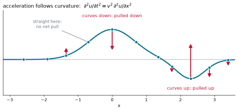

Fig. A snapshot of a string. Each arrow is the acceleration of a bead, proportional to the local curvature: downward on the crest, upward in the trough, zero where the string is straight.

Combining waves: interference¶

We are often interested in the result of several waves acting together, which is described mathematically by adding the waves.
Adding two solutions of the wave equation produces another solution. This is the principle of linear superposition: if $u_A$ and $u_B$ both solve the wave equation, so does $u_C = u_A + u_B$ . It holds because every term in the equation contains $u$ to the first power.
Interference is the name for what superposition looks like: the combined wave can have a greater, smaller, or unchanged amplitude depending on how the crests of the two waves line up.

Wave interference: derivation

Given the two waves

\Psi_1(x,t) = e^{i(kx - \omega t + \phi_1)}, \qquad \Psi_2(x,t) = e^{i(kx - \omega t + \phi_2)}

(18)

we want their sum $\Psi_{\text{total}} = \Psi_1 + \Psi_2$ .

Factor out the common exponential $e^{i(kx - \omega t)}$ :

\Psi_{\text{total}}(x,t) = e^{i(kx - \omega t)} \left( e^{i\phi_1} + e^{i\phi_2} \right)

(19)

Pull out the average phase. Write $\phi_1 = \bar\phi + \delta/2$ and $\phi_2 = \bar\phi - \delta/2$ with $\bar\phi = (\phi_1+\phi_2)/2$ and $\delta = \phi_1 - \phi_2$ :

e^{i\phi_1} + e^{i\phi_2} = e^{i \bar\phi} \left( e^{i \delta/2} + e^{-i \delta/2} \right)

(20)

Recognize a cosine. By Euler’s formula the bracket is $2\cos(\delta/2)$ :

e^{i \delta/2} + e^{-i \delta/2} = 2 \cos\left( \frac{\phi_1 - \phi_2}{2} \right)

(21)

Put it together:

\Psi_{\text{total}}(x,t) = 2 \cos\left( \frac{\phi_1 - \phi_2}{2} \right) e^{i \left( kx - \omega t + \frac{\phi_1 + \phi_2}{2} \right)}

(22)

Conclusion. The sum of two equal-amplitude waves is again a wave of the same $k$ and $\omega$ . Its phase is the average of the two phases and its amplitude is $2|\cos(\delta/2)|$ , where $\delta$ is the phase difference. The amplitude is 2 (constructive) for $\delta = 0$ and vanishes (destructive) for $\delta = \pi$ . A phase difference of $\pi/2$ gives $\sqrt{2}$ , in between.

Interference is what makes the double-slit pattern of Chapter 1. Two point sources oscillating in phase send out circular waves; along directions where the two paths differ by a whole number of wavelengths the crests arrive together and the waves reinforce, and where the paths differ by a half-integer number of wavelengths they cancel.

# synced: two_source_interference
import numpy as np
import matplotlib.pyplot as plt
from matplotlib.animation import FuncAnimation
from IPython.display import HTML

TEAL, CARDINAL, GRAY, PURPLE, ORANGE = "#107895", "#C8102E", "#6c757d", "#6a3d9a", "#e07b00"
plt.rcParams.update({"axes.spines.top": False, "axes.spines.right": False})
lam = 1.0; k, w = 2 * np.pi / lam, 2 * np.pi; d = 3 * lam
xs = np.linspace(-6, 6, 220); ys = np.linspace(0, 12, 220)
X, Y = np.meshgrid(xs, ys)
r1, r2 = np.hypot(X + d / 2, Y), np.hypot(X - d / 2, Y)
damp = lambda r: 1 / np.sqrt(1 + r)                     # gentle 2D spreading
ts = np.linspace(0, 2 * np.pi / w, 30, endpoint=False)
r1f, r2f = np.hypot(xs + d / 2, 12), np.hypot(xs - d / 2, 12)
I_far = np.abs(damp(r1f) * np.exp(1j * k * r1f) + damp(r2f) * np.exp(1j * k * r2f))**2

fig, (ax, bx) = plt.subplots(1, 2, figsize=(9, 4.4), gridspec_kw={"width_ratios": [1.15, 1]})
levels = np.linspace(-1.2, 1.2, 13)
ax.set_xlim(-6, 6); ax.set_ylim(0, 12); ax.set_aspect("equal")
ax.plot([-d / 2, d / 2], [0, 0], "o", color=CARDINAL, ms=8, mec="white", mew=1.2, clip_on=False, zorder=5)
ax.set_xlabel("x"); ax.set_ylabel("y")
ax.set_title(r"two in-phase point sources,  $d = 3\lambda$", loc="left", fontsize=11.5)
bx.plot(xs, I_far / I_far.max(), color=CARDINAL, lw=2.4)
bx.fill_between(xs, I_far / I_far.max(), color=CARDINAL, alpha=0.12)
bx.set_xlim(-6, 6); bx.set_ylim(0, 1.1)
bx.set_xlabel("x along the far edge  (y = 12)"); bx.set_ylabel("time-averaged intensity")
bx.set_title("bright and dark fringes", loc="left", fontsize=11.5)
fig.tight_layout()
art = []

def update(i):
    t = ts[i]
    for c in art:
        c.remove()
    art.clear()
    u = damp(r1) * np.cos(k * r1 - w * t) + damp(r2) * np.cos(k * r2 - w * t)
    art.append(ax.contourf(X, Y, u, levels=levels, cmap="RdBu_r", extend="both"))

ani = FuncAnimation(fig, update, frames=len(ts), interval=100, blit=False)
plt.close(fig)
HTML(ani.to_jshtml())

Fig. Left: two point sources (red dots) three wavelengths apart send out circular waves. The gray bands radiating outward are lines of destructive interference. Right: the time-averaged intensity along the top edge shows the bright and dark fringes of a double-slit pattern.

Move the sliders: the phase shift takes the red sum from double amplitude to zero, and the phasor panel shows why.

Standing waves from traveling waves¶

So far the two waves we added traveled in the same direction. Something new happens when two equal waves travel in opposite directions, which is exactly what happens on a string whose ends reflect the wave back. Using the identity $\sin a + \sin b = 2\sin\frac{a+b}{2}\cos\frac{a-b}{2}$ :

The result no longer contains the combination $x \mp vt$ ; space and time have separated into a product $X(x)\,T(t)$ . The shape $\sin(kx)$ stays put and only its overall height $2\cos(\omega t)$ oscillates.
Points where $\sin(kx)=0$ , that is $kx = n\pi$ or $x = n\lambda/2$ , never move at all. They are the nodes, spaced half a wavelength apart. Halfway between them sit the antinodes, where the string swings with the full amplitude $2A$ .

# synced: traveling_standing
import numpy as np
import matplotlib.pyplot as plt
from matplotlib.animation import FuncAnimation
from IPython.display import HTML

TEAL, CARDINAL, GRAY, PURPLE, ORANGE = "#107895", "#C8102E", "#6c757d", "#6a3d9a", "#e07b00"
plt.rcParams.update({"axes.spines.top": False, "axes.spines.right": False})
k, w = 1.0, 1.0                        # v = w/k = 1
x = np.linspace(0, 4 * np.pi, 800)     # two wavelengths
ts = np.linspace(0, 2 * np.pi / w, 36, endpoint=False)
nodes = np.arange(0, 4 * np.pi + 1e-9, np.pi / k)

fig, axes = plt.subplots(3, 1, figsize=(7.5, 5.6), sharex=True)
titles = [r"travels right:  $\sin(kx-\omega t)$", r"travels left:  $\sin(kx+\omega t)$",
          r"their sum:  $2\sin(kx)\cos(\omega t)$,  a standing wave"]
lines, dots = [], []
for ax, ttl, col in zip(axes, titles, [TEAL, ORANGE, CARDINAL]):
    (ln,) = ax.plot([], [], color=col, lw=2.4)
    (dt,) = ax.plot([], [], "o", color=col, ms=8, mec="white", mew=1.2)
    lines.append(ln); dots.append(dt)
    ax.axhline(0, color=GRAY, lw=0.6)
    ax.set_title(ttl, fontsize=11.5, loc="left", pad=4); ax.set_yticks([])
axes[0].set_ylim(-1.3, 1.3); axes[1].set_ylim(-1.3, 1.3); axes[2].set_ylim(-2.5, 2.5)
axes[2].plot(x, 2 * np.sin(k * x), color=GRAY, lw=1, ls="--")
axes[2].plot(x, -2 * np.sin(k * x), color=GRAY, lw=1, ls="--")
axes[2].plot(nodes, np.zeros_like(nodes), "o", color=GRAY, ms=7, zorder=5)
axes[2].text(nodes[1], -2.2, "nodes never move", color=GRAY, fontsize=10, ha="center")
axes[2].set_xlabel("x"); axes[2].set_xlim(0, 4 * np.pi)
axes[2].set_xticks(nodes)
axes[2].set_xticklabels(["0", r"$\lambda/2$", r"$\lambda$", r"$3\lambda/2$", r"$2\lambda$"])
fig.tight_layout()

def update(i):
    t = ts[i]
    lines[0].set_data(x, np.sin(k * x - w * t))
    lines[1].set_data(x, np.sin(k * x + w * t))
    lines[2].set_data(x, 2 * np.sin(k * x) * np.cos(w * t))
    dots[0].set_data([(np.pi / 2 + w * t) / k], [1.0])                 # a crest moving right
    dots[1].set_data([(np.pi / 2 + 2 * np.pi - w * t) / k], [1.0])     # a crest moving left
    dots[2].set_data([np.pi / (2 * k)], [2 * np.cos(w * t)])           # an antinode: up and down only

ani = FuncAnimation(fig, update, frames=len(ts), interval=85, blit=False)
plt.close(fig)
HTML(ani.to_jshtml())

Fig. Top and middle: equal waves traveling right and left; the dots ride along with a crest. Bottom: their sum is a standing wave. The gray nodes never move, the antinode (red dot) only moves up and down, and the dashed envelope $\pm 2\sin(kx)$ is the shape the string fills out.

If the string is clamped at both ends, the ends must be nodes. That single requirement selects the wavelengths that fit, $L = n\lambda/2$ , and leads to the discrete set of normal modes solved for in the next lecture. This is the same “waves have to fit” argument that quantized the Bohr orbits in Chapter 1.

Beats: waves of slightly different wavelength¶

One more superposition is worth seeing. Add two waves of equal amplitude but slightly different $k$ and $\omega$ , using $\cos a + \cos b = 2\cos\frac{a-b}{2}\cos\frac{a+b}{2}$ :

\cos(k_1x-\omega_1 t) + \cos(k_2x-\omega_2 t) = \underbrace{2\cos\!\Big(\frac{\Delta k}{2}x-\frac{\Delta\omega}{2}t\Big)}_{\text{slow envelope}} \;\underbrace{\cos\!\big(\bar k x-\bar\omega t\big)}_{\text{fast carrier}}

(24)

where $\bar k = (k_1+k_2)/2$ , $\Delta k = k_2-k_1$ , and likewise for $\omega$ .

The result is a fast wave at the average frequency whose amplitude is modulated by a slow envelope. The envelope repeats every $2\pi/\Delta k$ in space and pulses at the beat frequency $\Delta\nu = |\nu_2-\nu_1|$ in time. This is the wobble you hear when two guitar strings are almost, but not quite, in tune.

# synced: beats
import numpy as np
import matplotlib.pyplot as plt
from matplotlib.animation import FuncAnimation
from IPython.display import HTML

TEAL, CARDINAL, GRAY, PURPLE, ORANGE = "#107895", "#C8102E", "#6c757d", "#6a3d9a", "#e07b00"
plt.rcParams.update({"axes.spines.top": False, "axes.spines.right": False})
v = 1.0
k1, k2 = 4.0, 5.0
w1, w2 = v * k1, v * k2
x = np.linspace(0, 20, 1600)
ts = np.linspace(0, 2 * np.pi, 40, endpoint=False)     # common period of both waves

fig, (ax1, ax2) = plt.subplots(2, 1, figsize=(8, 4.8), sharex=True)
(l1,) = ax1.plot([], [], color=TEAL, lw=1.5, label=r"$\cos(k_1x-\omega_1t)$")
(l2,) = ax1.plot([], [], color=ORANGE, lw=1.5, label=r"$\cos(k_2x-\omega_2t)$")
ax1.set_ylim(-1.5, 1.7); ax1.set_yticks([])
ax1.legend(loc="upper right", frameon=False, fontsize=9.5, ncol=2)
ax1.set_title("two waves with slightly different wavelengths", loc="left", fontsize=11.5)
(ls,) = ax2.plot([], [], color=CARDINAL, lw=2.0, label="sum")
(e1,) = ax2.plot([], [], color=GRAY, lw=1.4, ls="--",
                 label=r"envelope $\pm 2\cos\left(\frac{\Delta k}{2}x - \frac{\Delta\omega}{2}t\right)$")
(e2,) = ax2.plot([], [], color=GRAY, lw=1.4, ls="--")
ax2.set_ylim(-2.7, 3.1); ax2.set_yticks([]); ax2.set_xlim(0, 20); ax2.set_xlabel("x")
ax2.legend(loc="upper right", frameon=False, fontsize=9.5, ncol=2)
ax2.set_title("their sum: a fast carrier inside a slow envelope (beats)", loc="left", fontsize=11.5)
for ax in (ax1, ax2):
    ax.axhline(0, color=GRAY, lw=0.6)
fig.tight_layout()

def update(i):
    t = ts[i]
    y1, y2 = np.cos(k1 * x - w1 * t), np.cos(k2 * x - w2 * t)
    l1.set_data(x, y1); l2.set_data(x, y2); ls.set_data(x, y1 + y2)
    env = 2 * np.cos(0.5 * (k2 - k1) * x - 0.5 * (w2 - w1) * t)
    e1.set_data(x, env); e2.set_data(x, -env)

ani = FuncAnimation(fig, update, frames=len(ts), interval=75, blit=False)
plt.close(fig)
HTML(ani.to_jshtml())

Fig. Two waves with $k_2/k_1 = 5/4$ (top) and their sum (bottom). Where the crests agree the sum is large, where they disagree it vanishes; the dashed envelope traces this slow modulation.

A wave you cannot surf: light and relativity¶

Our very first step was to ride along with the wave. A surfer moving at the wave speed $v$ sees a frozen shape, and the shore observer sees that shape slide by: $x = x' + vt$ . For water, sound, and strings this works because the wave lives in a medium, and “speed $v$ ” means speed relative to that medium.
Light is the exception. Maxwell’s equations of electromagnetism turn out to contain a wave equation for the electric and magnetic fields, with a speed built from two constants of nature and no medium in sight:

\frac{\partial^2 E}{\partial x^2} = \frac{1}{c^2}\frac{\partial^2 E}{\partial t^2}, \qquad c = \frac{1}{\sqrt{\varepsilon_0 \mu_0}} = 3.00\times 10^8\ \text{m/s}

(25)

With no medium there is nothing for “speed relative to the medium” to mean. At sixteen, Einstein asked what a light wave would look like if he could run alongside it at $c$ : a frozen electromagnetic ripple, which Maxwell’s equations do not allow. His resolution (1905) was to take the wave equation at its word: light moves at $c$ for every observer, however fast that observer moves. There is no surfer frame for light, and the everyday rule $x' = x - vt$ must fail at speeds near $c$ .
The simplest consequence shows up in a light clock: a photon bouncing between two mirrors a distance $d$ apart, one round trip per tick. At rest the tick lasts $\Delta t_0 = 2d/c$ . Now watch the same clock fly past at speed $v$ . The photon travels a longer zigzag path, but at the same speed $c$ , so each tick takes longer. Pythagoras on one half-tick, $(c\,\Delta t/2)^2 = d^2 + (v\,\Delta t/2)^2$ , gives:

# synced: light_clock
import numpy as np
import matplotlib.pyplot as plt
from matplotlib.animation import FuncAnimation
from IPython.display import HTML

TEAL, CARDINAL, GRAY, PURPLE, ORANGE = "#107895", "#C8102E", "#6c757d", "#6a3d9a", "#e07b00"
plt.rcParams.update({"axes.spines.top": False, "axes.spines.right": False})
c, v, d = 1.0, 0.6, 1.0                          # light speed, clock speed, mirror gap
gamma = 1 / np.sqrt(1 - v**2 / c**2)             # 1.25
T0 = 2 * d / c                                   # one tick of the clock at rest
ts = np.linspace(0, 3 * T0, 48, endpoint=False)  # three ticks of the rest clock
bounce = lambda tau: d * (1 - np.abs(2 * (tau % 1.0) - 1))   # 0 -> d -> 0 once per unit tau

fig, (ax, bx) = plt.subplots(1, 2, figsize=(9.5, 4.2), gridspec_kw={"width_ratios": [1, 2.4]})
for a_, xlim in ((ax, (-0.8, 0.8)), (bx, (-0.8, 4.4))):
    a_.set_xlim(*xlim); a_.set_ylim(-0.35, 1.45); a_.set_yticks([]); a_.set_xticks([])
    for s in ("left", "bottom"):
        a_.spines[s].set_visible(False)
(mir_a0,) = ax.plot([-0.5, 0.5], [0, 0], color="#333333", lw=5, solid_capstyle="butt")
(mir_a1,) = ax.plot([-0.5, 0.5], [d, d], color="#333333", lw=5, solid_capstyle="butt")
(ph_a,) = ax.plot([], [], "o", color=ORANGE, ms=13, mec="#ffd27f", mew=2.5, zorder=6)
(path_a,) = ax.plot([], [], color=ORANGE, lw=1.2, ls=":", alpha=0.8)
tick_a = ax.text(0, -0.25, "", ha="center", fontsize=12, color=TEAL, fontweight="bold")
ax.set_title(r"clock at rest:  tick $= 2d/c$", loc="left", fontsize=11.5)
ax.text(0.62, d / 2, "d", fontsize=12, color=GRAY, va="center")
ax.plot([0.58, 0.58], [0, d], color=GRAY, lw=1, marker="_", ms=8)

(mir_b0,) = bx.plot([], [], color="#333333", lw=5, solid_capstyle="butt")
(mir_b1,) = bx.plot([], [], color="#333333", lw=5, solid_capstyle="butt")
(ph_b,) = bx.plot([], [], "o", color=ORANGE, ms=13, mec="#ffd27f", mew=2.5, zorder=6)
(path_b,) = bx.plot([], [], color=ORANGE, lw=1.2, ls=":", alpha=0.8)
tick_b = bx.text(0, -0.25, "", ha="center", fontsize=12, color=CARDINAL, fontweight="bold")
bx.annotate("", xy=(4.2, 1.32), xytext=(2.9, 1.32), arrowprops=dict(arrowstyle="->", color=GRAY, lw=1.6))
bx.text(3.55, 1.37, "v = 0.6 c", color=GRAY, fontsize=10.5, ha="center")
bx.set_title(rf"moving at $v = 0.6c$:  longer path at the same $c$, tick $= \gamma\, 2d/c$,  $\gamma$ = {gamma:.2f}",
             loc="left", fontsize=11.5)
fig.suptitle("light moves at c for every observer, so the moving clock ticks slower", fontsize=12.5, y=0.99)
fig.tight_layout(rect=(0, 0, 1, 0.94))

def update(i):
    t = ts[i]
    tt = np.linspace(0, t, 300)
    ph_a.set_data([0], [bounce(t / T0)])
    path_a.set_data(np.zeros_like(tt), bounce(tt / T0))
    tick_a.set_text(f"ticks: {int(t // T0)}")
    xc = v * t
    mir_b0.set_data([xc - 0.5, xc + 0.5], [0, 0]); mir_b1.set_data([xc - 0.5, xc + 0.5], [d, d])
    ph_b.set_data([xc], [bounce(t / (gamma * T0))])
    path_b.set_data(v * tt, bounce(tt / (gamma * T0)))
    tick_b.set_position((xc, -0.25)); tick_b.set_text(f"ticks: {int(t // (gamma * T0))}")

ani = FuncAnimation(fig, update, frames=len(ts), interval=90, blit=False)
plt.close(fig)
HTML(ani.to_jshtml())

Fig. Left: a light clock at rest ticks every $2d/c$ . Right: the same clock moving at $v = 0.6c$ . The photon’s zigzag path is longer by $\gamma = 1.25$ , and since $c$ is unchanged the moving clock has completed fewer ticks at every instant.

Problems¶

Problem 1: Traveling or standing¶

Which of these functions can describe a traveling wave, and with what velocity: $u=(x+t)^2$ , $u=\cos(x-2t)$ , $u=\cos(x)\sin(t)$ ?

Solution

If a function can be cast in the form $f(x\pm vt)$ , it describes a wave propagating with constant velocity $v$ along the $x$ axis.

$u=(x+t)^2$ has the form $f(x+vt)$ with $v=1$ : a wave traveling in the negative $x$ direction with speed 1.
$u=\cos(x-2t)$ has the form $f(x-vt)$ with $v=2$ : a wave traveling in the positive $x$ direction with speed 2.
$u=\cos(x)\sin(t)$ cannot be written as a function of $x\pm vt$ alone: it is a product $X(x)T(t)$ , a standing wave.

Problem 2: Wavelength and frequency¶

Given the traveling wave $u(x,t) = \sin(2x-10t+\pi/2)$ in SI units, extract its amplitude, wavelength, angular frequency, frequency, period, and velocity.

Solution

Compare with the standard form $A\sin(kx-\omega t+\phi)$ and read off the constants:

$A=1$ , the multiplier in front of the sine.
$k=2\ \text{m}^{-1}$ , hence $\lambda = 2\pi/k = \pi\ \text{m} \approx 3.14\ \text{m}$ .
$\omega = 10\ \text{s}^{-1}$ , the coefficient of $t$ . Hence $\nu = \omega/2\pi = 5/\pi \approx 1.59\ \text{Hz}$ and $T = 1/\nu = \pi/5 \approx 0.63\ \text{s}$ .
$v = \omega/k = 5\ \text{m/s}$ , in the positive $x$ direction because the argument has the form $kx-\omega t$ . Check: $\lambda\nu = \pi \cdot 5/\pi = 5\ \text{m/s}$ .
The phase $\phi = \pi/2$ turns the sine into a cosine: $\sin(\theta+\pi/2) = \cos\theta$ , so $u = \cos(2x-10t)$ .

Problem 3: Checking the wave equation by the chain rule¶

A. Show by direct differentiation that the Gaussian pulse $u(x,t) = e^{-(x-vt)^2}$ satisfies the classical wave equation.
B. Does $u(x,t) = x^2 - v^2t^2$ satisfy it?

Solution

A. Let $s = x-vt$ , so $u = e^{-s^2}$ and $\dfrac{du}{ds} = -2s\,e^{-s^2}$ , $\dfrac{d^2u}{ds^2} = (4s^2-2)\,e^{-s^2}$ .

By the chain rule, $\partial s/\partial x = 1$ and $\partial s/\partial t = -v$ , so

\frac{\partial^2 u}{\partial x^2} = \frac{d^2u}{ds^2}, \qquad \frac{\partial^2 u}{\partial t^2} = (-v)^2\frac{d^2u}{ds^2} = v^2\frac{d^2u}{ds^2}.

(27)

Therefore $\dfrac{\partial^2 u}{\partial x^2} = \dfrac{1}{v^2}\dfrac{\partial^2 u}{\partial t^2}$ , as required. Nothing about the Gaussian was used: any $f(x-vt)$ passes the same test.

B. Here $\partial^2 u/\partial x^2 = 2$ while $\partial^2 u/\partial t^2 = -2v^2$ , so the right-hand side of the wave equation is $-2 \neq 2$ . It is not a solution. Note that $x^2-v^2t^2 = (x-vt)(x+vt)$ is a product of a right-moving and a left-moving function; the wave equation only guarantees that sums $f(x-vt)+g(x+vt)$ are solutions.

Problem 4: Reading a standing wave¶

A string carries the standing wave $u(x,t) = 0.02\,\sin(3.14\,x)\cos(62.8\,t)$ in SI units.

A. What are the wavelength, frequency, and speed of the two traveling waves it is made of?
B. How far apart are the nodes?

Solution

A. Compare with $2A\sin(kx)\cos(\omega t)$ : $k = 3.14\ \text{m}^{-1}$ so $\lambda = 2\pi/k = 2.0\ \text{m}$ ; $\omega = 62.8\ \text{s}^{-1}$ so $\nu = \omega/2\pi = 10\ \text{Hz}$ . Each underlying traveling wave has amplitude $A = 0.01\ \text{m}$ and speed $v = \omega/k = \lambda\nu = 20\ \text{m/s}$ , one moving right and one moving left.

B. Nodes are where $\sin(kx) = 0$ , at $x = n\pi/k = n\lambda/2 = 0,\ 1,\ 2,\ldots\ \text{m}$ . They are $\lambda/2 = 1.0\ \text{m}$ apart.

Problem 5: A red laser¶

A helium-neon laser emits light with $\lambda = 633\ \text{nm}$ . Find $k$ , $\nu$ , $\omega$ , and $T$ , and write the wave in complex form $Ae^{i(kx-\omega t)}$ with the numerical values of $k$ and $\omega$ in SI units. How many wavelengths fit in 1 mm?

Problem 6: Tuning by beats¶

Two guitar strings sound at 440 Hz and 444 Hz.

A. What beat frequency does a listener hear, and what is the period of the loudness pulsation?
B. Sound travels at 343 m/s. What are the two wavelengths, and over what distance in space does the beat envelope repeat?

Problem 7: Real and imaginary parts¶

Show that the real part and the imaginary part of $\Psi = Ae^{i(kx-\omega t)}$ each satisfy the classical wave equation separately. Which property of the wave equation guarantees this without any calculation?

Problem 8: Interference and standing waves by phasors¶

A. Two equal waves of amplitude $A$ interfere to give a wave of amplitude $1.2A$ . What is the phase difference between them? For what phase difference is the combined amplitude exactly $A$ ?
B. Use $\sin(a - b) = \sin a\cos b - \cos a\sin b$ to write the traveling wave $\sin(kx-\omega t)$ as a sum of two standing waves. How are the two standing waves shifted relative to each other in space and in time?

Problem 9: The light clock¶

A. Derive the time-dilation formula from the light clock: while a photon makes one round trip between mirrors a distance $d$ apart, the clock moves a distance $v\,\Delta t$ . Apply Pythagoras to one half of the trip.
B. At what speed does a moving clock run at half the rate of a clock at rest?
C. Muons created high in the atmosphere live $2.2\ \mu\text{s}$ in their own frame and move at $0.998c$ . How far do they travel before decaying, with and without time dilation? (Without it almost none would reach the ground; they do.)