Diffraction, interference and the double-slit experiment
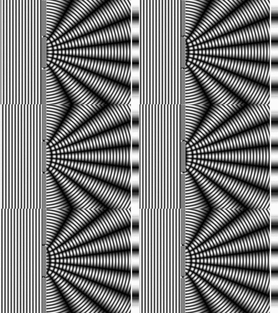
Figure 1:Waves passing through two slits create a diffraction pattern on the screen.
Diffraction: spreading of waves around obstacles or through small openings. Diffraction can occur with any type of wave, including light, sound, radio, and water.
Interference: when two waves meet, their combined intensity goes up or down depending on whether the waves are in phase or out of phase, respectively.
Double-slit experiment: light waves (or water waves) pass through a wall with two slits, which results in wave-like interference patterns, or bands, on the detector screen.
Bragg’s formula for diffraction
X-rays interact with the atoms in a crystal. The phase shift upon scattering off of atoms causes constructive (left figure) or destructive (right figure) interferences.
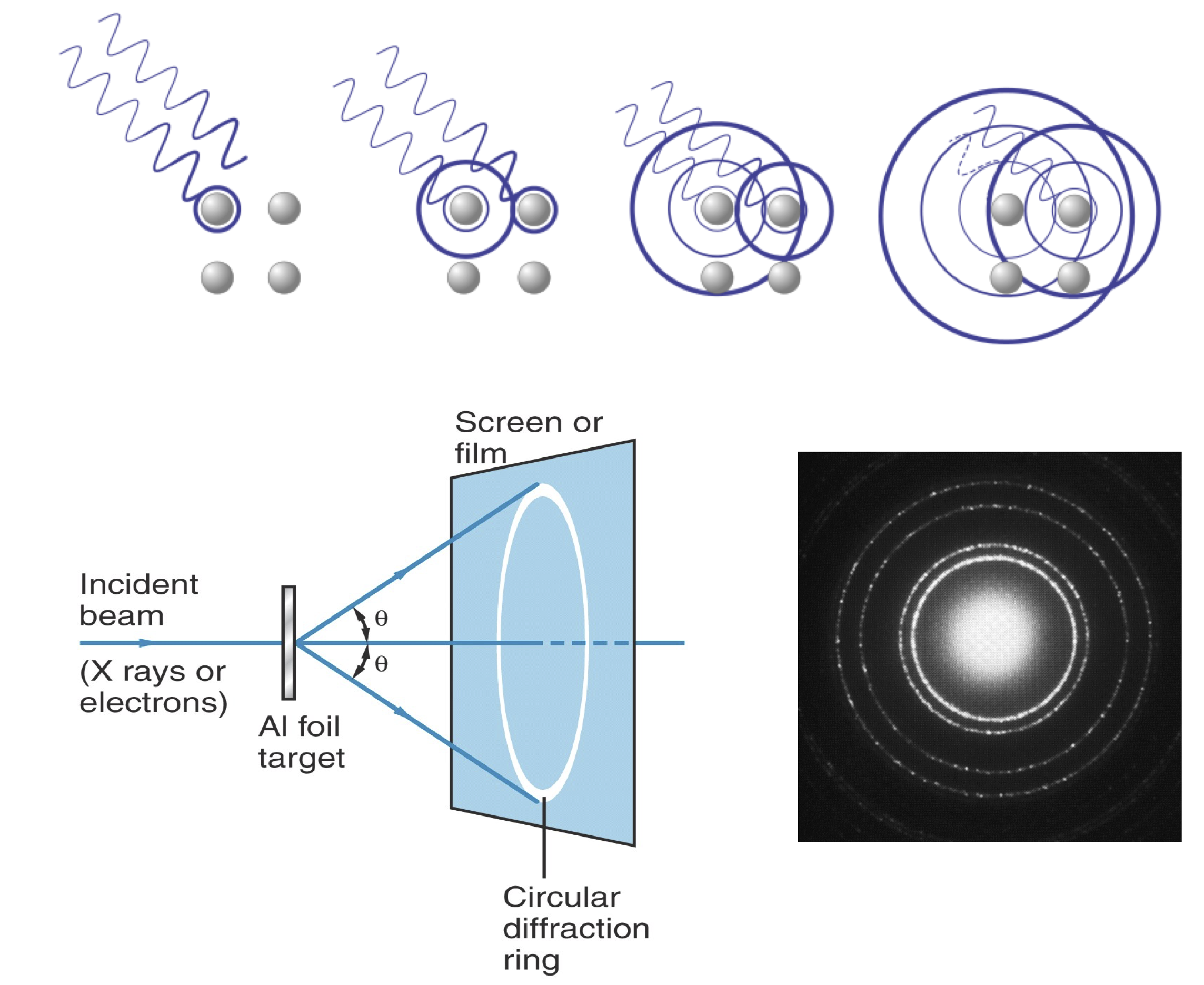
Figure 2:X-rays scattering off atoms in a crystal: constructive interference (left) and destructive interference (right).
Maxima and minima in interference patterns arise from simple geometry, as captured by Bragg’s law:
: spacing between atomic planes in the lattice
: wavelength of the radiation
: order of diffraction. For , the extra path length is one wavelength; for , it is two wavelengths, and so on. Higher-order reflections () occur at larger angles and are usually weaker, so in practice most analyses focus on .
Waves such as X-rays produce interference patterns according to this relation. Historically, such interference was regarded as a hallmark of wave-like behavior.
Both X-rays and electrons show diffraction patterns
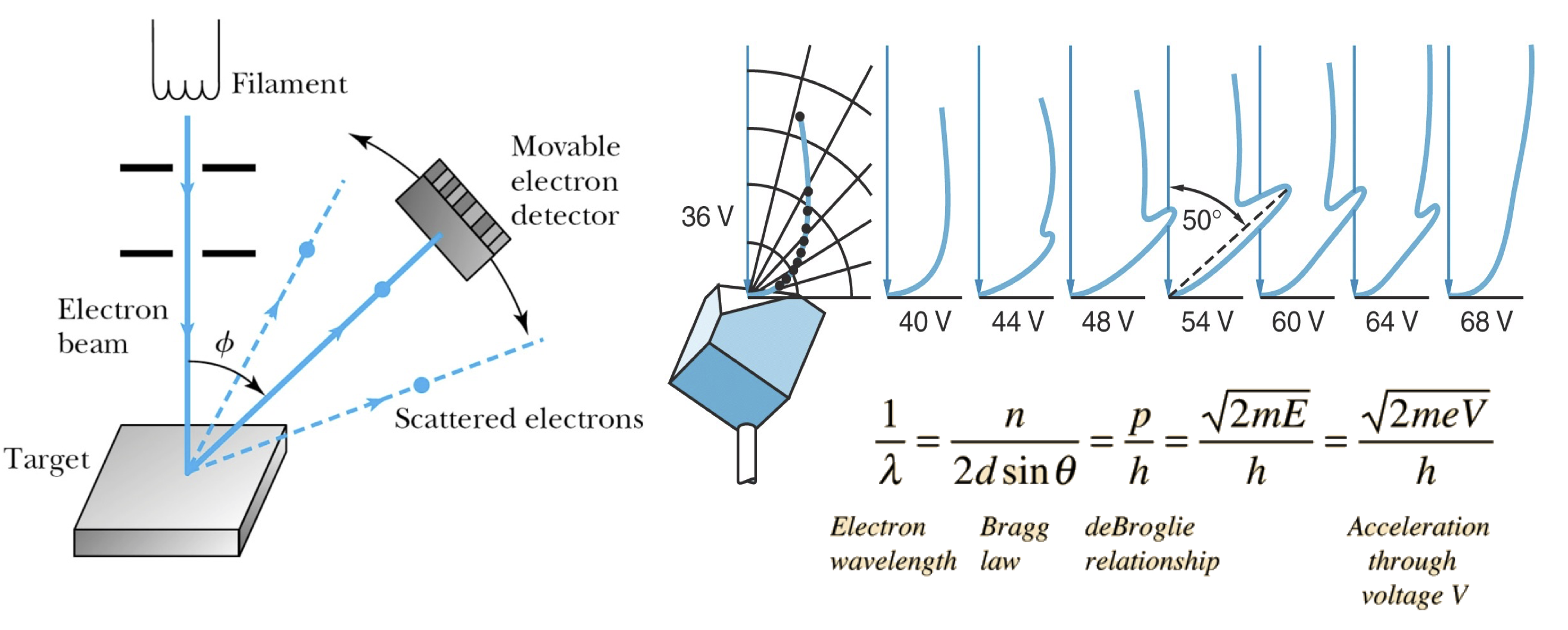
Figure 3:Demonstration of electron diffraction.
In 1927, Davisson and Germer were studying electron scattering from various materials. To their great surprise, they discovered that at certain angles there was a peak in the intensity of the scattered electron beam.
This peak indicated wave behavior for the electrons and could be interpreted by Bragg’s law (previously only applied to X-ray scattering) to give values for the lattice spacing in the nickel crystal.
Compton scattering
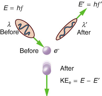
Figure 4:Compton scattering: photons scatter off electrons just as massive particles do.
Arthur Compton showed that X-rays get scattered off free electrons like elastic billiard balls. Applying conservation of momentum principle (previously only applied to particle-like objects), it was shown that the outgoing X-rays should be of longer wavelength than the incoming ones.
This means that a moving photon hits the resting free electron and transfers some energy to get the electron moving. Note that this experimental result makes sense only if you think of a photon as a particle with linear momentum which gets bounced off the electron.
De Broglie wavelength and wave-particle duality
Light is a wave and a particle. An electron is also a particle and a wave. Is everything a wave and a particle? The answer is YES! This is what is meant by wave-particle duality. Sometimes we only see one side of the duality because, under certain conditions, either the wave or the particle characteristics are more pronounced.
The wave-like and particle-like characteristics of a physical entity are inversely proportional to each other as described by the de Broglie relationship.
The relation implies that heavy objects have a small wavelength, and light objects have a large wavelength.
The smaller the object, the more pronounced wave-like qualities it will have. And vice versa, the bigger the object, the more particle-like qualities it will have.
Effect of potential energy
According to classical physics, the total energy for a particle is given as a sum of the kinetic and potential energies:
If we substitute de Broglie’s expression for momentum we get:
This equation shows that the de Broglie wavelength of a particle such as an electron with constant total energy changes as it moves into a region with different potential energy.
This has implications for chemical bonding, where electrons experience different fields in atoms and molecules.
Waves have to fit
The de Broglie relation has a consequence that goes far beyond diffraction. Take the electron wave and wrap it around a closed loop, as in an orbit around a nucleus. After one complete trip around the loop, called a pass, the wave meets itself and has no choice but to agree with where it started. If the circumference holds a whole number of wavelengths, every pass reinforces the one before it and a standing wave survives. If it does not, successive passes land out of step and the wave interferes itself away.
Source
import numpy as np
import matplotlib.pyplot as plt
from matplotlib.animation import FuncAnimation
from matplotlib.patches import Circle
from IPython.display import HTML

TEAL, CARDINAL, GRAY, PURPLE, GREEN = "#107895", "#C8102E", "#6c757d", "#6a3d9a", "#1a7f37"
R, AMP, LAPS = 1.0, 0.17, 8              # ring radius, wave amplitude, passes summed
th1 = np.linspace(0, 2 * np.pi, 900)             # first pass around the loop
th2 = np.linspace(2 * np.pi, 4 * np.pi, 900)     # second pass around the loop

# amplitude left after LAPS passes: the passes add as phasors exp(2 pi i n k)
n_grid = np.linspace(1.5, 6.5, 2000)
survival = np.abs(np.exp(2j * np.pi * n_grid * np.arange(LAPS)[:, None]).sum(axis=0)) / LAPS

n_seq = [2.0] * 4                        # sweep n, pausing on each whole number
for target in (3.0, 4.0, 5.0, 6.0):
    n_seq += list(np.linspace(n_seq[-1], target, 11, endpoint=False)) + [target] * 4

fig, (ax, bx) = plt.subplots(1, 2, figsize=(8.8, 4.2), gridspec_kw={"width_ratios": [1, 1.15]})

ax.add_patch(Circle((0, 0), R, fill=False, color=GRAY, lw=1.2, ls="--"))
ax.plot(0, 0, "o", color=CARDINAL, ms=9)
(lap1,) = ax.plot([], [], color=PURPLE, lw=2.4, label="1st pass")
(lap2,) = ax.plot([], [], color="#e07b00", lw=2.0, ls="--", label="2nd pass")
(gap,) = ax.plot([], [], color=CARDINAL, lw=3.4, solid_capstyle="butt", zorder=6)
(startdot,) = ax.plot([], [], "o", color=PURPLE, ms=8, mec="white", mew=1.2, zorder=7)
(enddot,) = ax.plot([], [], "o", color="#e07b00", ms=8, mec="white", mew=1.2, zorder=7)
gaplabel = ax.text(0, -1.42, "", fontsize=10.5, ha="center", va="center")
verdict = ax.set_title("", fontsize=12, pad=10)
ax.legend(loc="lower center", bbox_to_anchor=(0.5, -0.12), ncol=2, frameon=False, fontsize=9)
ax.set_xlim(-1.5, 1.5); ax.set_ylim(-1.5, 1.55); ax.set_aspect("equal"); ax.axis("off")

bx.plot(n_grid, survival, color=TEAL, lw=2.2)
bx.fill_between(n_grid, survival, color=TEAL, alpha=0.10)
(marker,) = bx.plot([], [], "o", color=CARDINAL, ms=9, zorder=5)
vline = bx.axvline(2.0, color=CARDINAL, lw=1.2, ls=":")
bx.set_xlim(1.5, 6.5); bx.set_ylim(-0.03, 1.18); bx.set_xticks(range(2, 7))
bx.set_xlabel(r"wavelengths around the orbit,  $n = 2\pi r / \lambda$", fontsize=11)
bx.set_ylabel("amplitude left after 8 passes", fontsize=11)
bx.set_title(r"Only integer $n$ survives", fontsize=12, pad=10)
for s in ("top", "right"):
    bx.spines[s].set_visible(False)
fig.suptitle(r"A standing wave on a Bohr orbit:  $2\pi r = n\lambda = nh/p$", fontsize=13.5, y=0.99)
fig.tight_layout(rect=(0, 0, 1, 0.93))

def update(i):
    n = n_seq[i]
    lap1.set_data((R + AMP * np.sin(n * th1)) * np.cos(th1), (R + AMP * np.sin(n * th1)) * np.sin(th1))
    lap2.set_data((R + AMP * np.sin(n * th2)) * np.cos(th2), (R + AMP * np.sin(n * th2)) * np.sin(th2))
    r1 = R + AMP * np.sin(2 * np.pi * n)          # where the wave sits after one full pass
    gap.set_data([R, r1], [0, 0]); startdot.set_data([R], [0]); enddot.set_data([r1], [0])
    closes = abs(n - round(n)) < 1e-9
    off = abs(n - round(n))
    verdict.set_text(f"$n$ = {n:.2f}   " + ("the wave closes on itself" if closes else "the wave misses itself"))
    verdict.set_color(GREEN if closes else CARDINAL)
    gaplabel.set_text("the 2nd pass lands on the 1st" if closes else rf"the 2nd pass is {off:.2f}$\lambda$ out of step")
    gaplabel.set_color(GREEN if closes else CARDINAL)
    marker.set_data([n], [abs(np.exp(2j * np.pi * n * np.arange(LAPS)).sum()) / LAPS])
    vline.set_xdata([n, n])
    return lap1, lap2, gap, startdot, enddot, gaplabel, marker, vline, verdict

ani = FuncAnimation(fig, update, frames=len(n_seq), interval=80, blit=False)
plt.close(fig)
HTML(ani.to_jshtml())Fig. Left: an electron wave wrapped around an orbit, drawn for two passes. Right: the amplitude left after eight passes, which is sharply peaked at whole numbers of wavelengths.
The closure condition is nothing more than the circumference holding wavelengths:
Rearranging gives the quantization of angular momentum,
Double-slit experiment
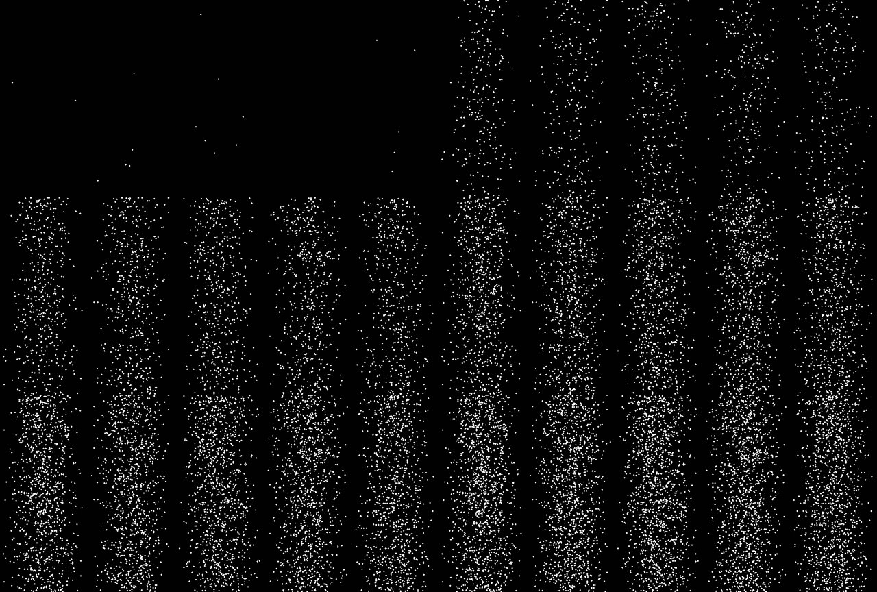
Figure 5:Wave-particle duality in the double-slit experiment.
Electron displays wave-like interference
The interference pattern arises only if we consider electrons as waves that interfere with each other (i.e., constructive and destructive interference).
When the experiment is carried out many times with only one electron going through the slits at a time, we still observe the interference effect.
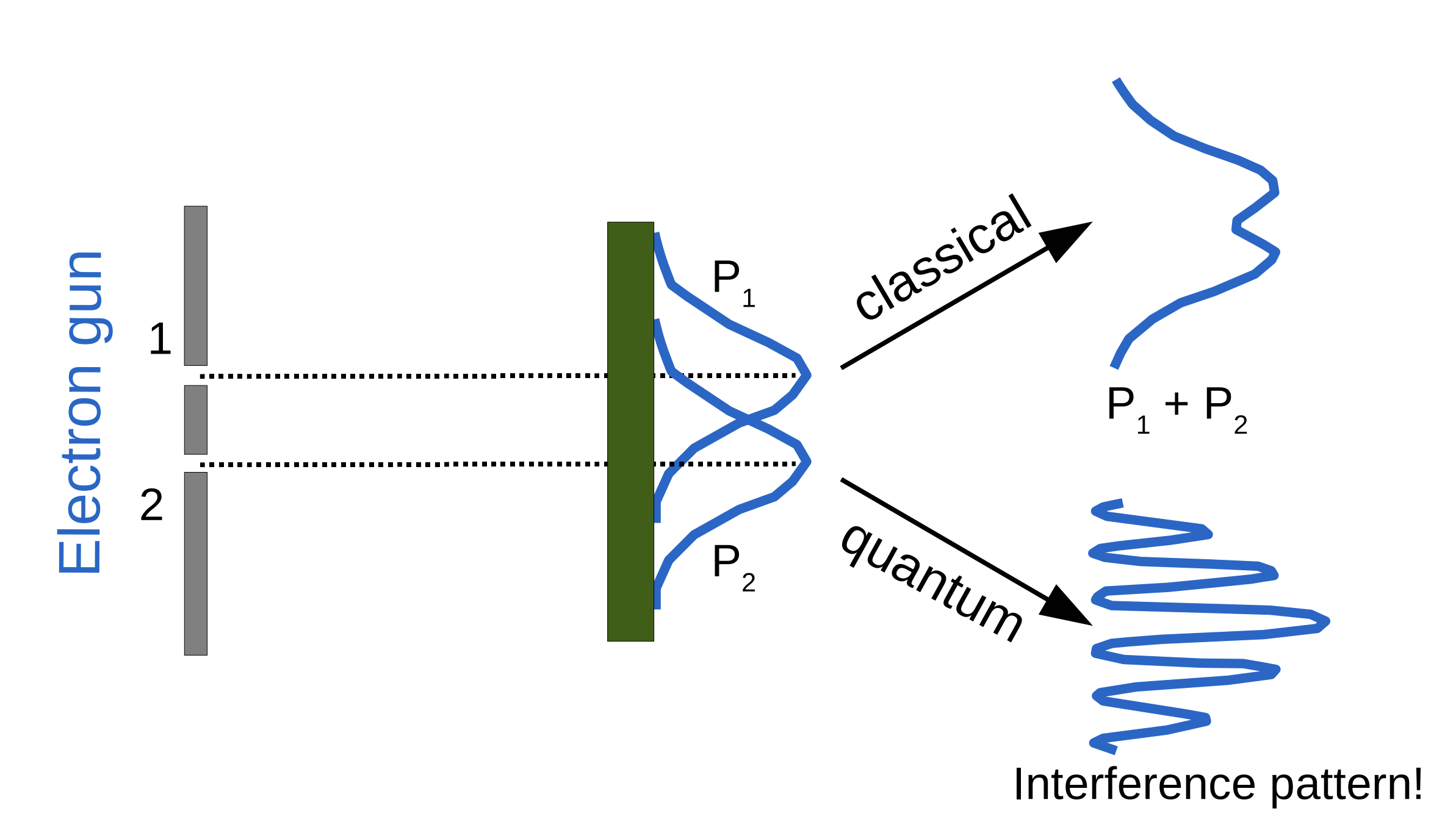
Figure 6:Where electrons are expected to land according to classical versus quantum theory.
But which slit did the electron go through??
If we try to determine which way the electron traveled, the interference pattern disappears!
We will return to resolve this puzzle after establishing the formal theory of quantum mechanics and its postulates.
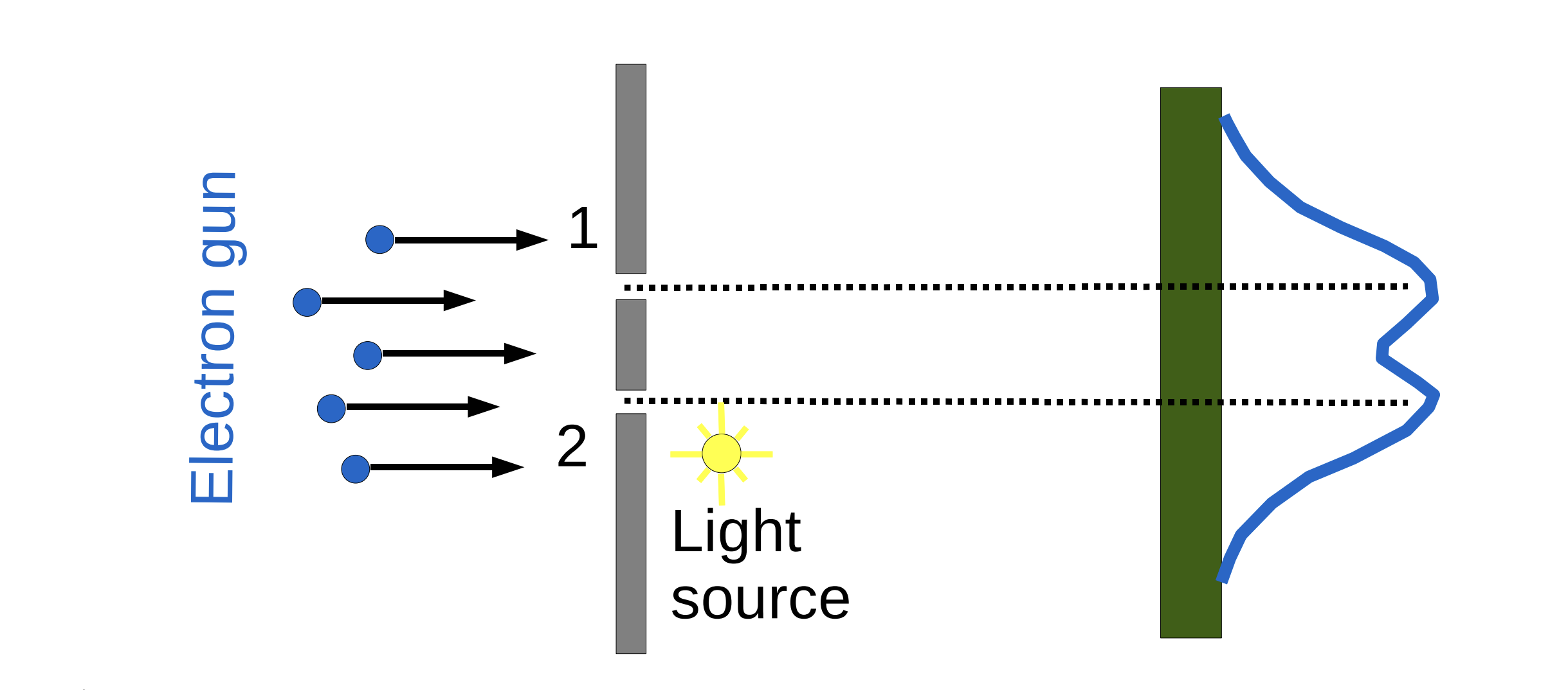
Figure 7:A detector fires photons to determine which slit each electron exits from.
Uncertainty relation
The uncertainty principle, also known as Heisenberg’s uncertainty principle, states that it is impossible to measure the exact position and momentum of a particle at the same time. This principle is based on the wave-particle duality of matter.
The principle states that the more precisely the position is known, the more uncertain the momentum is, and vice versa. For example, if we know everything about where a particle is located, we know nothing about its momentum.
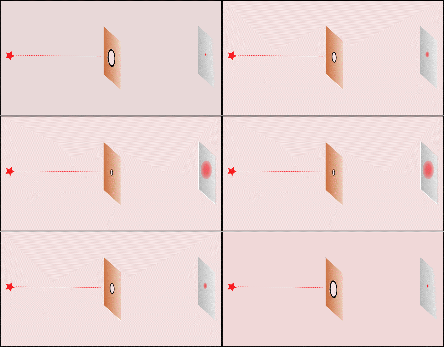
Figure 8:Demonstration of the uncertainty principle. As the electron’s position is localized by narrowing the slit, its momentum becomes more unpredictable, so the electrons hit the detector over a wider range.
Mathematically, the uncertainty relation is expressed in terms of the standard deviations of position and momentum , which are obtained by repeating the experiment, measuring positions and momenta, and quantifying the spread via the standard deviation.
Problems
Problem 1: Electrons in an electron microscope
Estimate the wavelength of electrons that have been accelerated from rest through a potential difference of .
Note that the potential energy difference the electrons experience is simply , where is the magnitude of the electron charge and is the potential difference.
Solution
Problem 2: Your own de Broglie wavelength
If you considered yourself a particle moving at , what would your de Broglie wavelength be? Would it make sense to use quantum mechanics in this case?
Solution
A. If you consider yourself a particle moving at , we can calculate your de Broglie wavelength using the de Broglie relation:
where is Planck’s constant, , and is the momentum of the object. The momentum is given by:
where is your mass and is your velocity. Assuming your mass is , the momentum would be:
Now, plugging the values into the de Broglie relation:
B. This wavelength is extremely small, much smaller than the scale at which quantum effects become noticeable. In this case, it wouldn’t make sense to use quantum mechanics, as classical mechanics is sufficient for describing the behavior of macroscopic objects like a person.
Problem 3: Position uncertainty in the Bohr atom
Quantify the uncertainty in the position of an electron in the ground state of the H atom using Bohr’s model.
Solution
To quantify the uncertainty in the position of an electron in the ground state of a hydrogen atom using Bohr’s model, we begin by recalling that the electron orbits the nucleus at a distance equal to the Bohr radius in the ground state. The Bohr radius is given by:
where:
(permittivity of free space),
(reduced Planck’s constant),
(mass of the electron),
(elementary charge).
Substituting these values, we can calculate the Bohr radius:
Now, Bohr’s model treats the electron as orbiting at this radius with a known trajectory. However, quantum mechanics introduces the Heisenberg uncertainty principle, which relates the uncertainties in position and momentum:
In the ground state, the uncertainty in momentum can be estimated from the momentum of the electron. The momentum of the electron in the Bohr model is related to the velocity and the mass :
Using the fact that the electron in the ground state has a velocity , we can calculate the momentum:
Now, using the uncertainty relation:
Substituting , we get:
Thus, the uncertainty in the position of the electron in the ground state of a hydrogen atom is approximately , which is on the order of the Bohr radius.
This result suggests that the electron’s position is spread out over a region approximately the size of the atom, supporting the idea that the electron in an atom cannot be described as a classical particle with a well-defined position.
Problem 4: Position uncertainty of a free electron
Quantify the uncertainty in the position of an electron traveling freely with a kinetic energy of .
Solution
To quantify the uncertainty in the position of an electron traveling freely with a kinetic energy of 3 eV, we can use the Heisenberg uncertainty principle:
First, we need to calculate the momentum of the electron. The kinetic energy is related to the momentum by the equation:
where:
(since ),
is the mass of the electron.
Rearranging for momentum:
Substituting the values:
Now, using the Heisenberg uncertainty principle:
Assuming , we substitute the values:
Thus, the uncertainty in the position of the electron traveling with a kinetic energy of 3 eV is approximately meters.
This is on the order of atomic scales, which indicates that quantum effects are relevant in this case.
Problem 5: Compton shift
X-rays from a molybdenum source ( pm) scatter off electrons in a graphite target. Compute the wavelength of the photons scattered at 90 degrees and at 180 degrees. What fraction of the photon energy is handed to the electron in the 180 degree case? Explain why the Compton shift is unobservable with visible light.
Problem 6: Thermal neutrons see atoms
Neutrons in equilibrium with a moderator at 300 K have an average kinetic energy of . Compute their de Broglie wavelength ( kg) and compare it with a typical spacing of atoms in a crystal, about 0.2 nm. Explain why neutron diffraction is used to locate hydrogen atoms in crystals when X-ray diffraction struggles.
Problem 7: Are helium atoms waves?
A beam of helium atoms leaves a nozzle at 300 K with a speed of about 1750 m/s. Compute the de Broglie wavelength of the atoms. In 1930 Estermann and Stern diffracted such a beam from a LiF crystal surface. Of the objects met so far (electron, X-ray photon, neutron, helium atom, a walking person), which show diffraction in practice, and what single quantity decides it?
Problem 8: Confinement costs energy
An electron is confined to a region the size of an atom, nm. (a) Use the uncertainty relation to find the minimum spread in momentum. (b) Taking , estimate the electron’s kinetic energy in eV. (c) Repeat for a proton confined to a nucleus, m, and give the result in MeV. What does the comparison say about the energy scales of chemistry versus nuclear physics?