Angular Momentum and Term Symbols - Quantum Mechanics for Chemistry

What you will learn

Total orbital angular momentum $\hat{L} = \sum_{i=1}^N \hat{l}_i$ quantifies the combined angular momentum of all electrons, with quantized values of $L$ ranging from $|l_1 - l_2|$ to $l_1 + l_2$ .
Total spin angular momentum $\hat{S} = \sum_{i=1}^N \hat{s}_i$ follows a similar quantization rule, with possible $S$ values for two electrons being 1 (triplet) or 0 (singlet).
The total angular momentum $\hat{J} = \hat{L} + \hat{S}$ combines orbital and spin contributions, with $J$ taking values from $|L - S|$ to $L + S$ .
Term symbols are written as $^{2S+1}L_J$ , where $2S+1$ is the spin multiplicity, $L$ is the total orbital momentum (S, P, D, F, ...), and $J$ is the total angular momentum.
Hund’s rules state that (1) the highest spin multiplicity lies lowest in energy, (2) for the same $S$ , the highest $L$ is lowest, and (3) for the same $S$ and $L$ , the smallest $J$ is lowest for a less-than-half-filled subshell, while the largest $J$ is lowest for a more-than-half-filled subshell.
Spin-orbit interaction couples $\vec{L}$ and $\vec{S}$ via $\hat{H}_{SO} = A\,\vec{\hat{L}} \cdot \vec{\hat{S}}$ , causing fine-structure splitting, especially in heavier atoms.
Selection rules for allowed transitions are $\Delta l = \pm 1$ , $\Delta L = 0, \pm 1$ (except $L = 0 \to L = 0$ ), $\Delta J = 0, \pm 1$ (except $J = 0 \to J = 0$ ), and $\Delta S = 0$ .
In light atoms, Russell-Saunders ( $LS$ ) coupling applies, so $L$ , $S$ , and $J$ are all good quantum numbers; in heavier atoms spin-orbit coupling dominates and $J$ becomes the only good quantum number.
The ground-state term symbol of an atom is determined using Hund’s rules; for example He ( $1s^2$ ) has term symbol $^1$ S $_0$ , while C ( $1s^2 2s^2 2p^2$ ) has term symbol $^3$ P $_0$ .

The Vector Model for Adding Angular Momenta¶

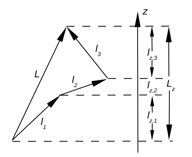
Vector addition of angular momenta — Fig. 1 Vector addition model used to determine the quantization of total angular momentum from individual contributions.

In many-electron atoms, each electron has both orbital and spin angular momenta. First, for simplicity, consider only the total orbital angular momentum operator:

{\hat{L} = \sum\limits_{i=1}^{N} \hat{l}_i}

(1)

where $N$ is the number of electrons and $\hat{l}_i$ is the angular momentum operator for electron $i$ . The projection operator along the $z$ -axis is then:

{\hat{L}_z = \sum\limits_{i=1}^{N} \hat{l}_{z,i}}

(2)

{M_L = \sum\limits_{i=1}^{N}m_i}

(3)

$\vec{L}$ is the total orbital angular momentum.
$\vec{l}_1, \vec{l}_2, \vec{l}_3$ are the individual angular momenta.
$\hat{L}, \hat{l}_i$ are operators; $L, l_i$ are the corresponding quantum numbers.
We assume a light atom and thus neglect the spin-orbit coupling.

Total Orbital Angular Momentum¶

Consider an atom with two electrons having orbital angular momenta $l_1$ and $l_2$ . The maximum total angular momentum is obtained when the two vectors are parallel: $L = l_1 + l_2$ . When they point in opposite directions, $L = |l_1 - l_2|$ . Hence the total angular momentum quantum number $L$ can take values (the “Clebsch-Gordan series”):

For example, if we have two electrons in $p$ -orbitals, this gives $L = 2, 1$ , or 0. Furthermore, for $L = 2$ we can have $M_L = +2, +1, 0, -1, -2$ ; for $L = 1$ , $M_L = +1, 0, -1$ ; and for $L = 0$ , $M_L = 0$ .

It is instructive to check that we have the same number of states in both representations (the uncoupled versus the coupled representation). In the uncoupled representation there are $3^2 = 9$ states (3 $p$ -orbitals and 2 electrons), and in the coupled representation $5 + 3 + 1 = 9$ .

Usually the closed-shell inner-core electrons are not included in the consideration, as they do not contribute to the end result.

Total Spin Angular Momentum¶

The total spin angular momentum operator for a many-electron atom is:

{\hat{S} = \sum\limits_{i=1}^{N}\hat{s}_i}

(5)

and the $z$ -component of the total spin operator is:

{\hat{S}_z = \sum\limits_{i=1}^{N}\hat{s}_{z,i}}

(6)

Here $\hat{s}_i$ and $\hat{s}_{z,i}$ refer to the spin angular momenta of the individual electrons. The total quantum number $M_S$ is:

{M_S = \sum\limits_{i=1}^{N} m_{s,i}}

(7)

This value ranges from $-S$ to $S$ , and the total quantum number $S$ is given by:

For example, for two electrons, $S = 1$ (a “triplet state”) or $S = 0$ (a “singlet state”).

Total Angular Momentum (Combined Orbital and Spin)¶

The total angular momentum operator $\hat{J}$ is the vector sum of $\hat{L}$ and $\hat{S}$ :

{\vec{\hat{J}} = \vec{\hat{L}} + \vec{\hat{S}}}

(9)

{\hat{J}_z = \hat{L}_z + \hat{S}_z}

(10)

The total quantum number $J$ , with its corresponding magnetic quantum number $M_J$ , is given by:

The coupling scheme above is called the $LS$ coupling or Russell-Saunders coupling.

This approach is only approximate when spin-orbit coupling is included in the Hamiltonian. Spin-orbit interaction arises from relativistic effects; here we simply think of it as coupling the orbital and spin angular momenta with some given magnitude (the “spin-orbit coupling constant”).

The spin-orbit effect is larger for heavier atoms. For these atoms the $LS$ coupling scheme begins to break down and only $J$ remains a good quantum number. This means, for example, that one can no longer speak about singlet and triplet electronic states. The $LS$ coupling scheme works reasonably well for the first two rows of the periodic table.

Atomic Terms and Selection Rules¶

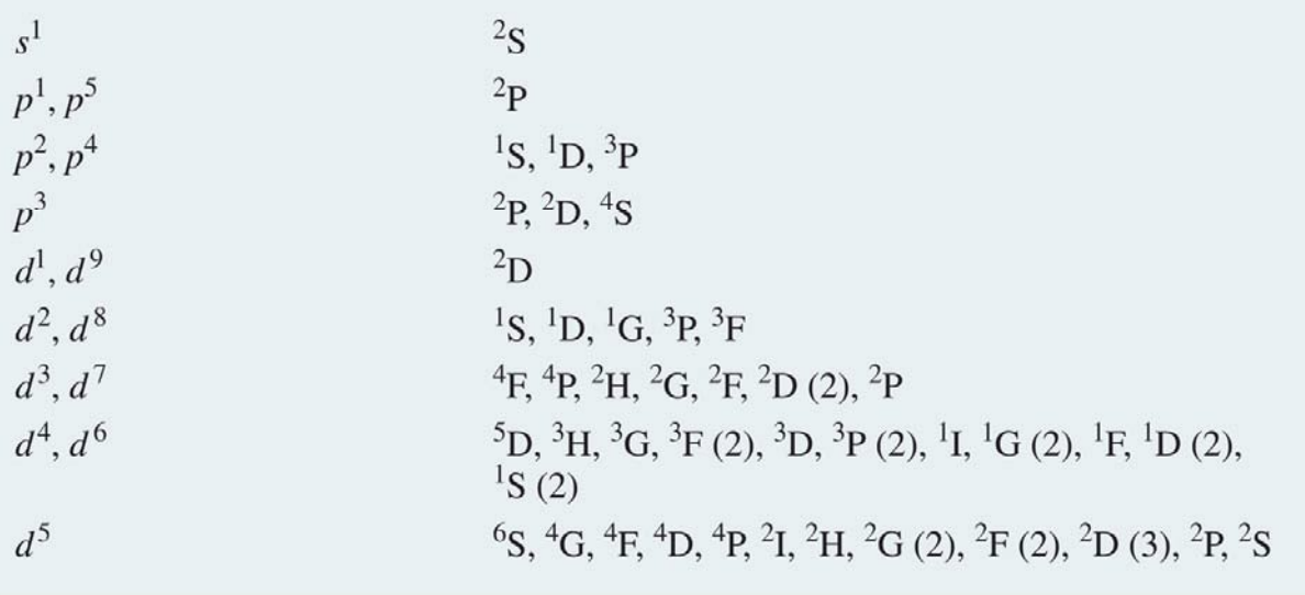
Fig. 2 Possible atomic terms for given electronic configurations.

The table above shows the various term symbols that can correspond to given electronic configurations. A term symbol contains information about the total orbital and spin angular momenta as well as the total angular momentum ( $J = L + S$ ):

Both $2S+1$ and $J$ are written as numbers, while $L$ is written as a letter: S for $L = 0$ , P for $L = 1$ , D for $L = 2$ , and so on. The quantity $2S+1$ is the spin multiplicity (1 = singlet, 2 = doublet, 3 = triplet, ...).

The term symbol specifies the ground-state electronic configuration exactly. Note that only the valence electrons contribute to the term symbol.

Because of electron, electron interactions and spin-orbit coupling, we expect a splitting of energy levels that can be described by various term symbols.

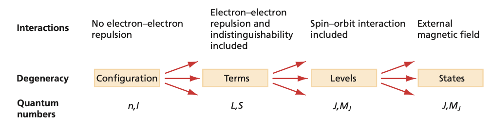
Configurations, terms, levels, states — Fig. 3 Relationship of configurations, terms, levels, and states. The top row indicates the degree of approximation and type of interaction; the second row shows the group of states that are degenerate in energy; and the bottom row indicates the good quantum numbers at each level of approximation.

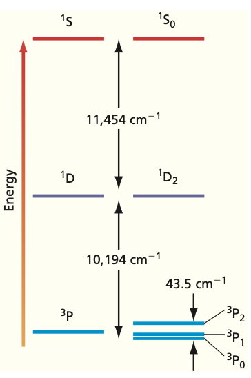
Term and level splitting of carbon — Fig. 4 Relationship of terms and levels for carbon. Assuming a spherically symmetric electron distribution, a single energy state is allowed. Including the dependence of electron repulsion on the directions of $L$ and $S$ splits this into terms of different energy, here $^3$ P, $^1$ D, and $^1$ S. Coupling of $L$ and $S$ further splits the terms into levels according to $J$ , here $^1$ S $_0$ , $^1$ D $_2$ , $^3$ P $_2$ , $^3$ P $_1$ , and $^3$ P $_0$ . The separation of the levels for the $^3$ P term has been multiplied by a factor of 25 to make it visible.

Example: lowest-lying terms of carbon

What are the lowest-lying term symbols for a carbon atom?

Solution

The electronic configuration for ground-state C is $1s^2 2s^2 2p^2$ . To get the possible lowest-lying states, we consider only the two $p$ -electrons. From the spin rule we get $S = \tfrac{1}{2} + \tfrac{1}{2} = 1$ or $S = 0$ . The first case corresponds to a triplet, the second to a singlet. The total orbital angular momentum quantum numbers are $L = 2, 1, 0$ , which correspond to D, P, and S terms, respectively. Because the electrons must have opposite spins when they share the same orbital, some $S$ and $L$ combinations are not allowed:

$L = 2$ (D term): One state ( $M_L = -2$ ) must have both electrons in the $p$ -orbital with $m_l = -1$ . These electrons must have opposite spins, so the triplet (parallel spins) is not allowed. Hence for $L = 2$ only the singlet $^1$ D is possible.
$L = 1$ (P term): In principle these configurations could also be written for the singlet, but a more careful analysis shows that this is not allowed.
$L = 0$ (S term): Here only $M_L = 0$ is possible. Again the triplet is not possible because the spins would have to be parallel in the same orbital, so only $^1$ S exists.

We conclude that the possible terms are $^1$ D, $^3$ P, and $^1$ S. Hund’s rules (below) predict that the $^3$ P term is the ground state. The total angular momentum quantum number $J$ for this state may be $J = L + S = 2, 1$ , or 0. Due to spin-orbit coupling these states have different energies, and Hund’s rules predict that the $J = 0$ state lies lowest. Therefore the $^3$ P $_0$ state is the ground state of the carbon atom.

The “ $L, S$ ” method above is fast and convenient but does not always work and cannot show, for instance, that $^1$ P does not exist. A more complete approach lists every possible electron configuration (microstate), labels each by its $M_L$ and $M_S$ values, counts how many times each $(M_L, M_S)$ combination appears, and decomposes the result into term symbols. The total number of microstates $N$ is:

{N = \frac{(2(2l+1))!}{n!\,(2(2l+1) - n)!}}

(14)

where $n$ is the number of electrons and $l$ is the orbital angular momentum quantum number (1 for $p$ -orbitals, 2 for $d$ , and so on). Counting the $(M_L, M_S)$ combinations and decomposing them into term symbols confirms the carbon result and shows explicitly that $^1$ P does not exist.

Hund’s Rules¶

Hund’s (partly empirical) rules are:

The term arising from the ground configuration with the maximum multiplicity $2S+1$ lies lowest in energy.
For levels with the same multiplicity, the one with the maximum value of $L$ lies lowest in energy.
For levels with the same $S$ and $L$ but different $J$ , the lowest-energy state depends on how much the subshell is filled:
- If the subshell is less than half-filled, the state with the smallest $J$ is lowest in energy.
- If the subshell is more than half-filled, the state with the largest $J$ is lowest in energy.

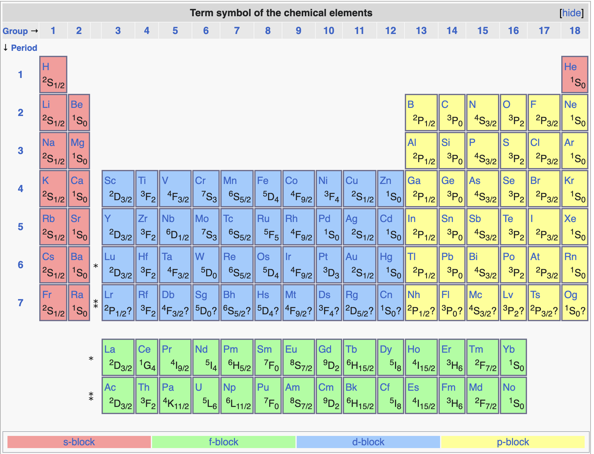
Ground-state terms across the periodic table — Fig. 5 Term symbols for the ground states of the elements across the periodic table.

Spin-Orbit Interaction¶

This relativistic effect can be incorporated into non-relativistic quantum mechanics by adding the following term to the Hamiltonian:

{\hat{H}_{SO} = A\,\vec{\hat{L}}\cdot \vec{\hat{S}}}

(15)

where $A$ is the spin-orbit coupling constant and $\hat{L}$ and $\hat{S}$ are the orbital and spin angular momentum operators.

The total angular momentum $J$ commutes with both $\hat{H}$ and $\hat{H}_{SO}$ , so it can be specified simultaneously with the energy. We say that the quantum number $J$ remains good even when spin-orbit interaction is included, whereas $L$ and $S$ do not. The operator dot product $\hat{L}\cdot\hat{S}$ can be evaluated in terms of the quantum numbers:

For example, in alkali atoms ( $S = 1/2$ , $L = 1$ ) the spin-orbit interaction breaks the degeneracy of the excited $^2$ P state into $^2$ P $_{3/2}$ and $^2$ P $_{1/2}$ (with $^2$ S $_{1/2}$ as the ground state).

Atomic Spectra and Selection Rules¶

The following selection rules for photon absorption or emission in one-electron atoms can be derived by considering the symmetries of the initial and final state wavefunctions:

{\Delta n = \textnormal{unrestricted},\quad \Delta l = \pm 1,\quad \Delta m_l = +1, 0, -1}

(17)

where $\Delta n$ is the change in the principal quantum number, $\Delta l$ the change in orbital angular momentum, and $\Delta m_l$ the change in its projection.

Qualitatively, the selection rules follow from conservation of angular momentum:

Photons are spin-1 particles with $m_l = +1$ (left-circularly polarized light) or $m_l = -1$ (right-circularly polarized light).
When a photon interacts with an atom, the angular momentum may change only by +1 or -1, exactly as in the selection rules above.

Selection Rules for Multi-Electron Atoms¶

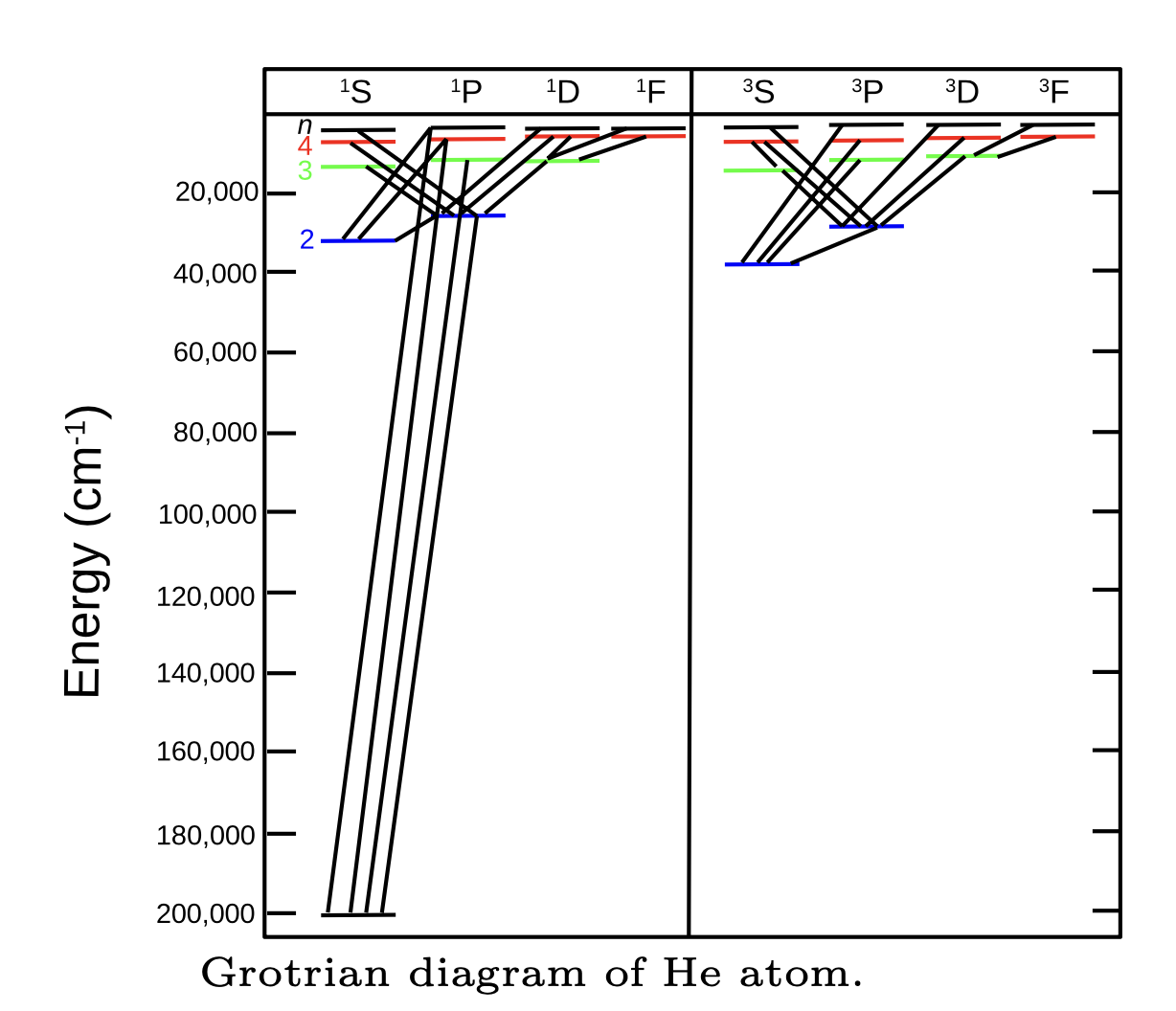
Allowed transitions of helium — Fig. 6 Allowed electronic transitions of the He atom, organized by term symbol.

$\Delta L = 0, \pm 1$ , except that a transition from $L = 0$ to $L = 0$ does not occur.
$\Delta l = \pm 1$ for the electron that is being excited (or is responsible for fluorescence).
$\Delta J = 0, \pm 1$ , except that a transition from $J = 0$ to $J = 0$ does not occur.
$\Delta S = 0$ : the electron spin does not change in an optical transition. The opposite holds for magnetic resonance spectroscopy, which deals with changes in spin states.

In some exceptional cases these rules may be violated, but the resulting transitions are extremely weak (“forbidden transitions”). Because of the last rule, some excited triplet states can have very long lifetimes, since the transition to the ground singlet state is forbidden (metastable states).

The Nature of Light, Matter Interaction¶

Light is electromagnetic radiation, so it has both electric and magnetic components. The oscillating electric field drives transitions in optical spectroscopy (UV/Vis, fluorescence, IR), whereas the magnetic component drives transitions in magnetic resonance spectroscopy (NMR, EPR/ESR).

Photon emission from an atom (for example, fluorescence) is difficult to understand with the quantum mechanical machinery developed so far. The plain Schrodinger equation predicts that excited states in atoms would have infinite lifetime in vacuum. This is not observed in practice: atoms and molecules return to the ground state by emitting a photon. This transition is caused by fluctuations of the electromagnetic field in the vacuum.

Problems¶

Problem 1: Spin multiplicity of two electrons

Two electrons each have spin $s = \tfrac{1}{2}$ . Use the spin-coupling rule to enumerate the allowed values of the total spin quantum number $S$ , the corresponding spin multiplicities $2S+1$ , and the allowed values of $M_S$ for each. Show that the total number of spin states is 4.

Solution

The coupling rule gives $S = s_1 + s_2, \ldots, |s_1 - s_2| = 1, 0$ .

$S = 1$ (triplet, $2S+1 = 3$ ): $M_S = +1, 0, -1$ , giving 3 states.
$S = 0$ (singlet, $2S+1 = 1$ ): $M_S = 0$ , giving 1 state.

The total is $3 + 1 = 4$ , which matches the $2^2 = 4$ states of the uncoupled representation ( $\alpha\alpha$ , $\alpha\beta$ , $\beta\alpha$ , $\beta\beta$ ).

Problem 2: Ground-state term symbol of nitrogen

Determine the ground-state term symbol of the nitrogen atom, whose valence configuration is $2p^3$ . Apply Hund’s rules in order.

Solution

With three $p$ -electrons and three $p$ -orbitals, the maximum-multiplicity arrangement (Hund’s first rule) puts one electron in each orbital with parallel spins:

M_S^{\max} = \tfrac{1}{2}+\tfrac{1}{2}+\tfrac{1}{2} = \tfrac{3}{2} \;\Rightarrow\; S = \tfrac{3}{2},\quad 2S+1 = 4.

(18)

With one electron in each of $m_l = +1, 0, -1$ , the total $M_L = +1+0-1 = 0$ , so $L = 0$ (an S term). The subshell is exactly half-filled, so the only value of $J$ is $J = L + S = \tfrac{3}{2}$ . The ground-state term symbol is $^4$ S $_{3/2}$ .

Problem 3: Spin-orbit splitting of a $^2$ P term

Using the eigenvalue of $\vec{\hat{L}}\cdot\vec{\hat{S}}$ , compute the spin-orbit energy $A\langle\vec{\hat{L}}\cdot\vec{\hat{S}}\rangle$ for the two levels $^2$ P $_{3/2}$ and $^2$ P $_{1/2}$ of an alkali atom ( $L=1$ , $S=\tfrac{1}{2}$ ). Which level lies lower for a less-than-half-filled subshell?

Solution

The eigenvalue is $\tfrac{1}{2}[J(J+1) - L(L+1) - S(S+1)]$ with $L(L+1) = 2$ and $S(S+1) = \tfrac{3}{4}$ .

$J = \tfrac{3}{2}$ : $\tfrac{1}{2}\left[\tfrac{15}{4} - 2 - \tfrac{3}{4}\right] = \tfrac{1}{2}(1) = +\tfrac{1}{2}$ , so $E_{SO} = +\tfrac{1}{2}A$ .
$J = \tfrac{1}{2}$ : $\tfrac{1}{2}\left[\tfrac{3}{4} - 2 - \tfrac{3}{4}\right] = \tfrac{1}{2}(-2) = -1$ , so $E_{SO} = -A$ .

For a less-than-half-filled subshell $A > 0$ , so the $J = \tfrac{1}{2}$ level lies lower, consistent with Hund’s third rule (smallest $J$ lowest).