Angular Momentum and Central Forces - Quantum Mechanics for Chemistry

Rotation is everywhere in chemistry: molecules tumble, bonds rotate, and electrons orbit nuclei. The classical mechanics of rotation, built on angular momentum and central forces, is the direct ancestor of two quantum models you will study: the rigid rotor and the hydrogen atom. This page develops that classical picture and points to where quantization enters.

Rotational motion and angular momentum¶

For a particle at position $\mathbf{r}$ with momentum $\mathbf{p} = m\mathbf{v}$ , the angular momentum about the origin is the cross product

For a mass moving in a circle of radius $r$ , $\mathbf{r}$ and $\mathbf{v}$ are perpendicular, so $L = mvr$ . Writing the speed as $v = \omega r$ with angular velocity $\omega$ gives $L = m r^2\omega = I\omega$ , where

I = mr^2

(2)

is the moment of inertia, the rotational analogue of mass. The rotational kinetic energy then mirrors the familiar $\tfrac{1}{2}mv^2$ :

The second form, energy as $L^2/2I$ , is the one that carries straight into the quantum rigid rotor.

import numpy as np
import matplotlib.pyplot as plt

theta = np.linspace(0, 2 * np.pi, 200)
R = 1.0
fig, ax = plt.subplots(figsize=(5.5, 5.5))
ax.plot(R * np.cos(theta), R * np.sin(theta), 'k', lw=1.5)  # orbit

# particle at 40 degrees, with r and v arrows
a = np.deg2rad(40)
pos = np.array([R * np.cos(a), R * np.sin(a)])
vel = np.array([-np.sin(a), np.cos(a)])  # tangent, counterclockwise
ax.annotate('', xy=pos, xytext=(0, 0),
            arrowprops=dict(arrowstyle='->', color='#2e4057', lw=2))
ax.annotate('', xy=pos + 0.6 * vel, xytext=pos,
            arrowprops=dict(arrowstyle='->', color='#d1495b', lw=2))
ax.plot(*pos, 'ko', ms=8)
ax.text(pos[0] * 0.5 - 0.15, pos[1] * 0.5, r'$\mathbf{r}$', color='#2e4057', fontsize=13)
ax.text(pos[0] + 0.6 * vel[0], pos[1] + 0.6 * vel[1] + 0.1, r'$\mathbf{v}$', color='#d1495b', fontsize=13)

# L out of plane, shown as a dot in a circle at the center
ax.plot(0, 0, 'o', ms=14, mfc='white', mec='#66a182', mew=2)
ax.plot(0, 0, 'o', ms=4, color='#66a182')
ax.text(0.12, 0.12, r'$\mathbf{L}$ (out of page)', color='#66a182', fontsize=11)

ax.set_xlim(-1.5, 1.7)
ax.set_ylim(-1.5, 1.7)
ax.set_aspect('equal')
ax.axhline(0, color='gray', lw=0.5)
ax.axvline(0, color='gray', lw=0.5)
ax.set_title(r'Fig.1 $\mathbf{L}=\mathbf{r}\times\mathbf{p}$ points out of the orbital plane')
plt.tight_layout()
plt.show()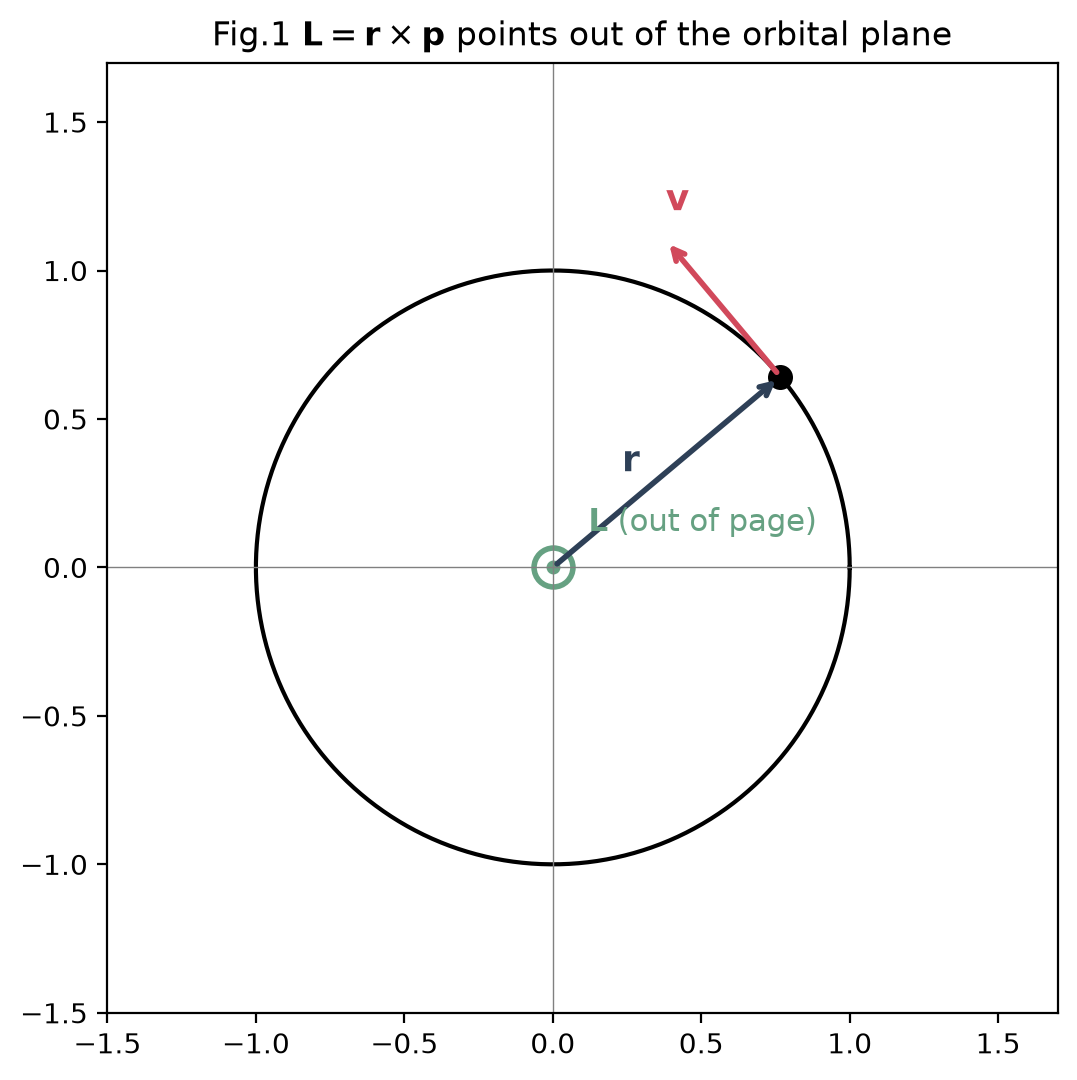

Torque and conservation¶

Just as force changes linear momentum, torque changes angular momentum:

A central force points along the line from the center to the particle, so $\mathbf{F}$ is parallel to $\mathbf{r}$ and their cross product vanishes. With zero torque, angular momentum is conserved:

\mathbf{F}\parallel\mathbf{r} \;\Longrightarrow\; \boldsymbol{\tau} = 0 \;\Longrightarrow\; \mathbf{L} = \text{constant}.

(5)

Gravity and the Coulomb attraction between an electron and a nucleus are both central, so both conserve angular momentum. This is why planetary orbits stay in a plane and sweep out equal areas in equal times (Kepler’s second law), and it is why the electron’s angular momentum is a good quantum number in the hydrogen atom.

Central forces and the effective potential¶

Because $\mathbf{L}$ is fixed, motion under a central force stays in a single plane, and the conserved $L$ can be folded into the energy. The radial motion then behaves like a one-dimensional problem in an effective potential:

The extra term $L^2/2mr^2$ is the centrifugal barrier: it grows without bound as $r\to 0$ , so a particle with any angular momentum is pushed away from the center and cannot fall in. For an attractive Coulomb potential $V(r) = -k/r$ the two terms compete, producing a minimum, a stable orbit at a preferred radius.

import numpy as np
import matplotlib.pyplot as plt

r = np.linspace(0.1, 8, 400)
k, m = 1.0, 1.0
V = -k / r

fig, ax = plt.subplots(figsize=(7, 4.5))
ax.plot(r, V, 'k--', lw=1.5, label=r'$V(r)=-k/r$ (attraction)')
for L, c in zip([0.8, 1.2, 1.6], ['#66a182', '#edae49', '#d1495b']):
    Veff = V + L**2 / (2 * m * r**2)
    ax.plot(r, Veff, color=c, lw=2, label=fr'$V_{{\rm eff}}$, L={L}')
    rmin = r[np.argmin(Veff)]
    ax.plot(rmin, np.min(Veff), 'o', color=c, ms=6)

ax.axhline(0, color='gray', lw=0.6)
ax.set_ylim(-1.2, 1.0)
ax.set_xlabel('radius r')
ax.set_ylabel('energy')
ax.legend(fontsize=9, loc='lower right')
ax.set_title('Fig.2 Centrifugal barrier creates a stable orbit (minimum) at larger L')
plt.tight_layout()
plt.show()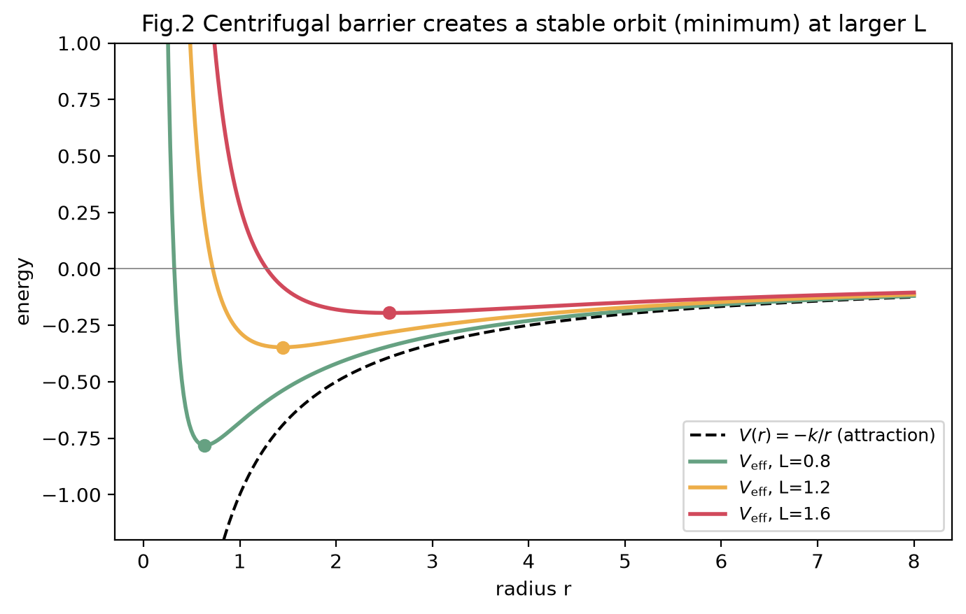

The minimum of each curve is a circular orbit; a particle with slightly more energy oscillates in $r$ between two turning points, tracing an ellipse. This effective-potential picture reappears almost unchanged in the radial Schrodinger equation for the hydrogen atom, where $L^2$ becomes the quantized $\hbar^2 l(l+1)$ .

Where quantization enters¶

Classically $L$ can take any value and point in any direction. Quantum mechanics restricts both.

The rigid rotor (Chapter 4). A molecule rotating with fixed bond length has energy $E = L^2/2I$ . Quantizing the angular momentum as $L^2 \to \hbar^2 J(J+1)$ gives the rotational ladder

E_J = \frac{\hbar^2}{2I}\,J(J+1), \qquad J = 0, 1, 2, \ldots

(7)

These are the levels probed by microwave (rotational) spectroscopy.

The hydrogen atom (Chapter 5). The electron feels the central Coulomb force, so its angular momentum is conserved and quantized. The magnitude is set by $l$ through $L = \hbar\sqrt{l(l+1)}$ , and its projection on an axis is set by $m$ through $L_z = \hbar m$ . This “space quantization” of a classically continuous vector is what gives orbitals their shapes and labels.

So the classical conservation law becomes a quantum number, and the classical effective potential becomes the radial equation. The rotational and orbital structure of matter is classical angular momentum, quantized.

Problems¶

Problem 1: Angular momentum of an orbit¶

A particle of mass $m = 2\ \text{kg}$ moves in a circle of radius $r = 3\ \text{m}$ at speed $v = 4\ \text{m/s}$ . Find $L$ and the moment of inertia $I$ .

Solution

L = mvr = 2\cdot 4\cdot 3 = 24\ \text{kg m}^2/\text{s}, \qquad I = mr^2 = 2\cdot 9 = 18\ \text{kg m}^2.

(9)

Check: $\omega = v/r = 4/3$ , and $I\omega = 18\cdot(4/3) = 24 = L$ .

Problem 2: Rotational energy two ways¶

For the particle in Problem 1, compute the rotational energy using both $\tfrac{1}{2}I\omega^2$ and $L^2/2I$ and confirm they agree.

Solution

\tfrac{1}{2}I\omega^2 = \tfrac{1}{2}(18)(4/3)^2 = 16\ \text{J}, \qquad \frac{L^2}{2I} = \frac{24^2}{2\cdot 18} = \frac{576}{36} = 16\ \text{J}.

(10)

Problem 3: Why no torque¶

Explain in one or two sentences why a central force conserves angular momentum.

Solution

A central force is parallel to $\mathbf{r}$ , so the torque $\boldsymbol{\tau} = \mathbf{r}\times\mathbf{F} = 0$ . Since $d\mathbf{L}/dt = \boldsymbol{\tau} = 0$ , the angular momentum is constant in magnitude and direction.

Problem 4: Rigid-rotor spacing¶

For the quantized rotor $E_J = \frac{\hbar^2}{2I}J(J+1)$ , find the energy gap between adjacent levels $J$ and $J+1$ .

Solution

\Delta E = E_{J+1} - E_J = \frac{\hbar^2}{2I}\big[(J+1)(J+2) - J(J+1)\big] = \frac{\hbar^2}{2I}\,2(J+1) = \frac{\hbar^2}{I}(J+1).

(11)

The gaps grow linearly with $J$ , so rotational spectral lines are evenly spaced by $\hbar^2/I$ .

Problem 5: Space quantization¶

For $l = 2$ , list the allowed values of $m$ and compute $L$ and the possible $L_z$ in units of $\hbar$ .

Problem 6: Centrifugal barrier¶

Explain, using the effective potential, why an electron with nonzero angular momentum cannot be found at the nucleus ( $r = 0$ ).

Problem 7: Kepler’s second law¶

Argue that constant angular momentum $L = mr^2\dot\phi$ implies the radius vector sweeps out equal areas in equal times, since the areal rate is $\tfrac{1}{2}r^2\dot\phi$ .