Electromagnetism and Light

Quantum mechanics was born from light: blackbody radiation, the photoelectric effect, and atomic spectra all involve light meeting matter. To see why those experiments forced quantization, we first need the classical picture of light as an electromagnetic wave. This page gives just enough electromagnetism to make those connections, ending at the door where the classical wave breaks down and the photon appears.

Electric and magnetic fields¶

A field assigns a vector to every point in space. The electric field $\mathbf{E}$ points along the force a positive charge would feel; the magnetic field $\mathbf{B}$ deflects moving charges sideways. Together they exert the Lorentz force on a charge $q$:

Everything about electricity, magnetism, and light comes down to how these two fields are made and how they change.

Maxwell’s equations¶

Maxwell collected four laws that, together, are complete: given the charges and currents, they fix the fields everywhere. In words and symbols:

The symbols $\nabla\cdot$ (divergence) and $\nabla\times$ (curl) measure how much a field spreads out from a point and how much it circulates around a point. You do not need to compute them here; the plain-language tags above carry the meaning. The two constants are the permittivity $\varepsilon_0$ and permeability $\mu_0$ of empty space.

The decisive feature is the coupling in the last two equations: a changing magnetic field creates an electric field, and a changing electric field creates a magnetic field. Each field feeds the other, and that feedback can travel.

From Maxwell to the wave equation¶

In empty space, with no charges ($\rho = 0$) or currents ($\mathbf{J} = 0$), the two curl equations feed back into each other. Taking the curl of Faraday’s law and substituting Ampere-Maxwell yields a wave equation for each field:

This is exactly the wave equation from Chapter 2, and its speed $c = 1/\sqrt{\mu_0\varepsilon_0} \approx 3.0\times10^8\ \text{m/s}$ is the measured speed of light. That numerical coincidence is what told Maxwell that light is an electromagnetic wave. Solving separately gives the same wave equation for $\mathbf{B}$, so electric and magnetic fields travel together.

A plane-wave solution has $\mathbf{E}$ and $\mathbf{B}$ oscillating in step, perpendicular to each other and to the direction of travel:

with wavenumber $k = 2\pi/\lambda$ and angular frequency $\omega = 2\pi\nu$.

Source

import numpy as np
import matplotlib.pyplot as plt

x = np.linspace(0, 4 * np.pi, 200)
E = np.cos(x)   # E along y
B = np.cos(x)   # B along z, in phase

fig = plt.figure(figsize=(9, 4))
ax = fig.add_subplot(111, projection='3d')

# Field curves
ax.plot(x, E, np.zeros_like(x), color='#d1495b', lw=2, label='E field (y)')
ax.plot(x, np.zeros_like(x), B, color='#2e4057', lw=2, label='B field (z)')

# A few field vectors as stems
for xi in x[::15]:
    ax.plot([xi, xi], [0, np.cos(xi)], [0, 0], color='#d1495b', lw=0.8, alpha=0.6)
    ax.plot([xi, xi], [0, 0], [0, np.cos(xi)], color='#2e4057', lw=0.8, alpha=0.6)

ax.plot(x, np.zeros_like(x), np.zeros_like(x), 'k', lw=1)  # propagation axis
ax.set_xlabel('propagation x')
ax.set_ylabel('E (y)')
ax.set_zlabel('B (z)')
ax.set_title('Fig.1 A plane electromagnetic wave: E and B perpendicular, oscillating in step')
ax.legend(fontsize=9, loc='upper right')
ax.view_init(elev=20, azim=-60)
plt.tight_layout()
plt.show()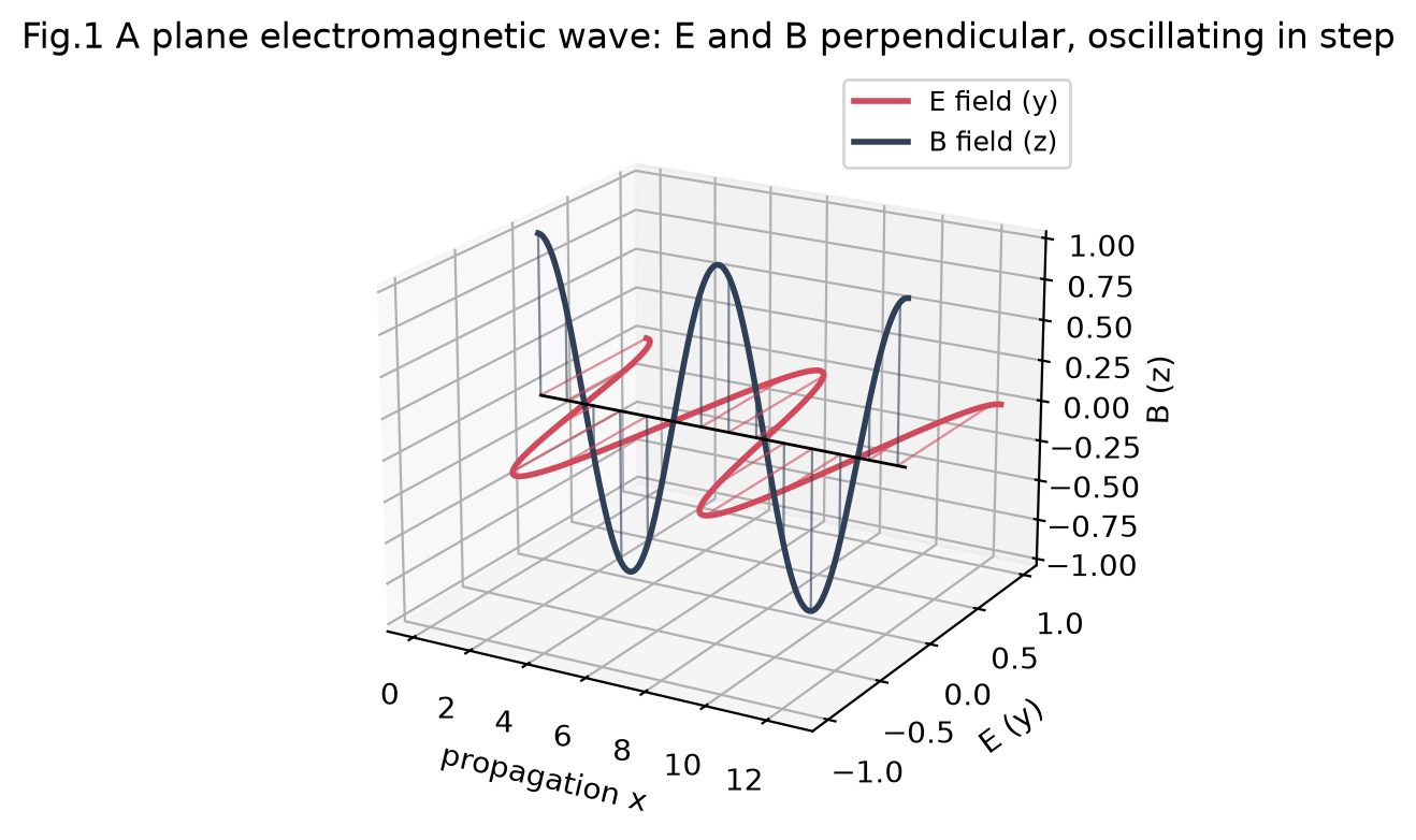

The electromagnetic spectrum¶

A single wave equation covers a vast range of wavelengths, all traveling at $c$ and related by

Radio waves, infrared, visible light, ultraviolet, and X-rays differ only in wavelength (and therefore frequency). Each region maps onto a kind of chemistry: rotations in the microwave, vibrations in the infrared, electronic transitions in the visible and ultraviolet.

Source

import numpy as np
import matplotlib.pyplot as plt

# Band edges in meters (approximate), plotted on a log-wavelength axis
bands = [
    ("Radio",     1e0,   1e-1, "#8ecae6"),
    ("Microwave", 1e-1,  1e-3, "#219ebc"),
    ("Infrared",  1e-3,  7e-7, "#d1495b"),
    ("Visible",   7e-7,  4e-7, "#66a182"),
    ("UV",        4e-7,  1e-8, "#8338ec"),
    ("X-ray",     1e-8,  1e-11, "#023047"),
]

fig, ax = plt.subplots(figsize=(9, 2.4))
for name, lam_hi, lam_lo, color in bands:
    left, width = np.log10(lam_lo), np.log10(lam_hi) - np.log10(lam_lo)
    ax.barh(0, width, left=left, height=0.6, color=color, edgecolor='white')
    ax.text(left + width / 2, 0, name, ha='center', va='center',
            fontsize=9, color='white', fontweight='bold')

ax.set_xlim(-11, 0.5)
ax.set_ylim(-0.6, 0.9)
ax.set_yticks([])
ax.set_xlabel(r'$\log_{10}(\lambda / \mathrm{m})$   (shorter wavelength, higher energy $\rightarrow$ to the left)')
ax.set_title('Fig.2 The electromagnetic spectrum, one wave equation across all wavelengths')
plt.tight_layout()
plt.show()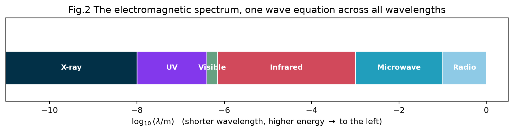

Where the classical picture breaks and quantum mechanics begins¶

Maxwell’s wave describes light perfectly until it exchanges energy with matter. Three experiments broke the classical picture and each is a chapter in this course:

• Blackbody radiation. The classical wave predicts infinite emission at short wavelengths (the “ultraviolet catastrophe”). Planck fixed it by letting light carry energy only in discrete lumps.

• The photoelectric effect. Light ejects electrons only above a threshold frequency, regardless of intensity, as if light arrives as particles of energy $E = h\nu$.

• Atomic spectra. Atoms absorb and emit light only at sharp frequencies, matching differences between quantized energy levels.

The unifying resolution is that light carries energy in quanta:

The classical field is still the right description of how light propagates and diffracts. What quantum mechanics adds is that energy is exchanged in packets, and that the same light-matter coupling, treated as a small perturbation, gives the selection rules of spectroscopy in Chapter 6. So this classical wave is not discarded; it is the backbone onto which quantization is grafted.

Problems¶

Problem 1: Wavelength to frequency¶

Green light has wavelength $\lambda = 500\ \text{nm}$. Find its frequency.

Problem 2: Photon energy¶

Find the energy of one photon of that green light, using $h = 6.63\times10^{-34}\ \text{J s}$.

Problem 3: The speed of light from constants¶

Given $\varepsilon_0 = 8.85\times10^{-12}\ \text{F/m}$ and $\mu_0 = 1.26\times10^{-6}\ \text{H/m}$, compute $c = 1/\sqrt{\mu_0\varepsilon_0}$.

Problem 4: Which Maxwell equation?¶

A changing magnetic flux through a loop of wire drives a current around it. Which of Maxwell’s equations describes this, and what is the effect called?

Problem 5: Spectroscopy mapping¶

Rank microwave, infrared, and ultraviolet photons by energy, and match each to the molecular motion it excites (rotation, vibration, electronic transition).

Problem 6: Verify the wave relation¶

A wave has $k = 2\pi/\lambda$ and $\omega = 2\pi\nu$. Show that the phase speed $\omega/k$ equals $\lambda\nu$.

Problem 7: Counting photons¶

A $1\ \text{mW}$ green laser ($\lambda = 500\ \text{nm}$) shines for one second. Roughly how many photons does it emit? Use the photon energy from Problem 2.