Classical Mechanics: From Newton to Hamilton - Quantum Mechanics for Chemistry

Before quantum mechanics we need one idea from classical physics done properly: the Hamiltonian. Newton’s laws are what you learned first, but quantum mechanics is not built on forces. It is built on energy, on the variables position and momentum, and on a bracket that becomes the commutator. This page explains why we reformulate classical mechanics and how that reformulation hands us the Schrodinger equation.

Newton’s mechanics¶

Newton’s second law says a force changes a particle’s momentum:

Give the force and the initial position and velocity, and the trajectory $x(t)$ is fixed for all time. For a mass on a spring the force is $F = -kx$ , giving oscillation $x(t) = A\cos(\omega t)$ with $\omega = \sqrt{k/m}$ .

Two quantities organize the motion. The kinetic energy $T = \tfrac{1}{2}mv^2$ and the potential energy $V(x)$ , whose negative slope is the force, $F = -dV/dx$ . Their sum, the total energy, stays constant as the particle moves:

E = T + V = \tfrac{1}{2}mv^2 + V(x) = \text{constant}.

(2)

Newton’s picture is intuitive, but it is awkward for quantum mechanics: it centers on force, a vector that is hard to generalize to abstract coordinates, and it hides the energy, which is the quantity quantum mechanics actually quantizes. We want a formulation built directly on energy.

The Hamiltonian reformulation¶

The trick is to stop using position and velocity, and instead use position $q$ and momentum $p = mv$ as the two independent variables. The Hamiltonian is the total energy written in terms of these:

All of the dynamics now follows from a single, strikingly symmetric pair of first-order equations:

The first equation just restates $p = m\dot q$ ; the second reproduces Newton’s law, since $-\partial H/\partial q = -dV/dq = F$ . So Hamilton’s equations contain exactly the same physics as $F = ma$ , only now written symmetrically in $q$ and $p$ and driven entirely by the energy function $H$ .

Where the Lagrangian fits

Between Newton and Hamilton sits the Lagrangian $L = T - V$ , whose Euler-Lagrange equation $\frac{d}{dt}\frac{\partial L}{\partial \dot q} = \frac{\partial L}{\partial q}$ follows from the principle of least action: the actual path makes the action $S = \int L\,dt$ stationary. The Hamiltonian is obtained from the Lagrangian by switching from velocity $\dot q$ to momentum $p = \partial L/\partial \dot q$ . We go straight to the Hamiltonian because it, not the Lagrangian, is what quantum mechanics quantizes. The least-action idea does return in Feynman’s path-integral formulation.

Phase space¶

In the Hamiltonian picture a complete classical state is a single point $(q, p)$ in phase space, the plane of position versus momentum. As time runs, the point moves along a curve, and because energy is conserved that curve is a contour of constant $H$ .

For the harmonic oscillator $H = \frac{p^2}{2m} + \frac{1}{2}m\omega^2 q^2$ , the constant-energy contours are ellipses. A low-energy state traces a small ellipse near the origin; higher energy means a bigger ellipse.

import numpy as np
import matplotlib.pyplot as plt

m, omega = 1.0, 1.0
q = np.linspace(-3, 3, 400)
p = np.linspace(-3, 3, 400)
Q, P = np.meshgrid(q, p)
H = P**2 / (2 * m) + 0.5 * m * omega**2 * Q**2

fig, axes = plt.subplots(1, 2, figsize=(11, 4.2))

# Phase-space energy contours (ellipses)
levels = [0.2, 0.5, 1.0, 1.8, 2.8]
cs = axes[0].contour(Q, P, H, levels=levels, cmap='viridis')
axes[0].clabel(cs, fmt='E=%.1f', fontsize=8)
# One trajectory, arrow shows clockwise flow
E = 1.0
theta = np.linspace(0, 2 * np.pi, 200)
axes[0].plot(np.sqrt(2 * E) * np.cos(theta), np.sqrt(2 * E) * np.sin(theta), 'k', lw=1)
axes[0].annotate('', xy=(np.sqrt(2 * E) * np.cos(0.3), np.sqrt(2 * E) * np.sin(0.3)),
                 xytext=(np.sqrt(2 * E), 0.0),
                 arrowprops=dict(arrowstyle='->', color='k'))
axes[0].set_xlabel('position q')
axes[0].set_ylabel('momentum p')
axes[0].set_aspect('equal')
axes[0].set_title('Fig.1a Phase space: energy contours are ellipses')

# Time view: position and momentum oscillate, 90 deg out of phase
t = np.linspace(0, 4 * np.pi, 400)
axes[1].plot(t, np.sqrt(2 * E) * np.cos(t), color='#2e4057', lw=2, label='q(t)')
axes[1].plot(t, -np.sqrt(2 * E) * np.sin(t), color='#d1495b', lw=2, label='p(t)')
axes[1].axhline(0, color='gray', lw=0.6)
axes[1].set_xlabel('time t')
axes[1].legend(fontsize=9)
axes[1].set_title('Fig.1b Newton view: q and p oscillate in time')

plt.tight_layout()
plt.show()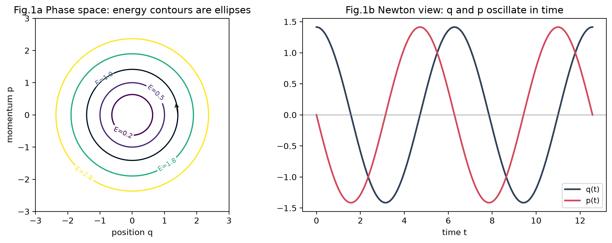

The two panels are the same motion in two languages: Hamilton’s phase-space ellipse (left) and Newton’s time trajectories (right). Quantum mechanics will replace the sharp phase-space point with a spread-out probability cloud, because position and momentum can no longer be pinned down at once.

Why the Hamiltonian is the bridge to quantum mechanics¶

Three features of the Hamiltonian formulation carry over almost verbatim into quantum mechanics.

Energy is the central object. Quantum mechanics quantizes energy, and $H$ is the energy. The quantum Hamiltonian $\hat H$ is what appears in the Schrodinger equation, and its eigenvalues are the allowed energy levels.

States and observables. A classical observable is any function of $(q, p)$ : position is $q$ , momentum is $p$ , energy is $H(q,p)$ . In quantum mechanics each becomes an operator, and the recipe (called canonical quantization) is direct:

Feeding this $\hat H$ into $i\hbar\,\partial_t\Psi = \hat H\Psi$ gives the Schrodinger equation. The classical Hamiltonian literally becomes the quantum Hamiltonian by substituting operators for $q$ and $p$ .

The Poisson bracket becomes the commutator. Classical mechanics has a bracket that measures how two observables co-vary,

\{A, B\} = \frac{\partial A}{\partial q}\frac{\partial B}{\partial p} - \frac{\partial A}{\partial p}\frac{\partial B}{\partial q}, \qquad \text{so}\quad \{q, p\} = 1.

(7)

Quantization promotes this bracket to the commutator through the rule $\{A,B\} \to \frac{1}{i\hbar}[\hat A, \hat B]$ , which turns $\{q,p\}=1$ into

This single non-zero commutator is the seed of the uncertainty principle: because $\hat x$ and $\hat p$ do not commute, no state can have a definite position and a definite momentum at the same time. The operators and differential equations page showed why non-commuting operators behave this way; here we see where that particular commutator comes from.

Problems¶

Problem 1: Recover Newton from Hamilton¶

For $H = \frac{p^2}{2m} + V(q)$ , apply Hamilton’s equations and show they combine into $m\ddot q = -dV/dq$ .

Solution

$\dot q = \partial H/\partial p = p/m$ , so $p = m\dot q$ . And $\dot p = -\partial H/\partial q = -dV/dq$ . Differentiating the first and substituting gives $m\ddot q = \dot p = -dV/dq$ , which is Newton’s law with $F = -dV/dq$ .

Problem 2: Hamiltonian of a falling body¶

Write the Hamiltonian for a mass $m$ in a uniform gravitational field, $V(z) = mgz$ , and use Hamilton’s equations to find $\dot p$ .

Solution

H = \frac{p^2}{2m} + mgz, \qquad \dot p = -\frac{\partial H}{\partial z} = -mg.

(10)

The momentum decreases at a constant rate, which is exactly $F = -mg$ .

Problem 3: Phase-space area¶

The harmonic-oscillator ellipse $\frac{p^2}{2m} + \frac{1}{2}m\omega^2 q^2 = E$ has semi-axes $\sqrt{2mE}$ in $p$ and $\sqrt{2E/m\omega^2}$ in $q$ . Show its enclosed area is $2\pi E/\omega$ .

Solution

The area of an ellipse is $\pi \times (\text{semi-axis}_1)\times(\text{semi-axis}_2)$ :

\pi\sqrt{2mE}\,\sqrt{\frac{2E}{m\omega^2}} = \pi\cdot\frac{2E}{\omega} = \frac{2\pi E}{\omega}.

(11)

Setting this area equal to $nh$ is the old Bohr-Sommerfeld quantization rule, and it reproduces $E_n = n\hbar\omega$ .

Problem 4: A Poisson bracket¶

Compute $\{q, H\}$ for $H = \frac{p^2}{2m} + V(q)$ and interpret the result.

Solution

\{q, H\} = \frac{\partial q}{\partial q}\frac{\partial H}{\partial p} - \frac{\partial q}{\partial p}\frac{\partial H}{\partial q} = \frac{p}{m} = \dot q.

(12)

The bracket with the Hamiltonian generates time evolution, the classical shadow of $\dot{\hat A} = \frac{i}{\hbar}[\hat H, \hat A]$ in quantum mechanics.

Problem 5: Quantize a free particle¶

Apply canonical quantization to the free-particle Hamiltonian $H = p^2/2m$ (no potential) and write the resulting $\hat H$ and time-independent Schrodinger equation.

Problem 6: Check the commutator¶

Using $\hat p = -i\hbar\,d/dx$ , act with $[\hat x, \hat p]$ on a test function $f(x)$ and confirm that $[\hat x, \hat p]f = i\hbar f$ .

Problem 7: Energy conservation¶

Show from Hamilton’s equations that $dH/dt = 0$ whenever $H$ has no explicit time dependence, so the total energy is conserved.