Statistical Mechanics and Blackbody Radiation - Quantum Mechanics for Chemistry

What you will learn

Temperature measures average energy. In a large collection of particles, energy is shared among many degrees of freedom, and temperature sets the average.
The equipartition theorem. Classically, every quadratic degree of freedom carries an average energy of $\tfrac{1}{2}k_BT$ .
The Boltzmann distribution. The probability of finding a system in a state of energy $E$ falls off as $e^{-E/k_BT}$ , which sets the populations of energy levels.
Blackbody radiation broke classical physics. Equipartition predicts an ultraviolet catastrophe; Planck’s quantized oscillators fixed it and launched quantum theory.
Populations drive spectroscopy. The intensity of a spectral line depends on how many molecules occupy the starting level, given by the Boltzmann factor.

Chemistry deals with moles of molecules, not single particles, so we need the physics of many particles sharing energy. That physics, statistical mechanics, does two jobs for this course. It exposes exactly where classical physics fails, in the blackbody spectrum, and it tells us how molecules populate energy levels, which is what every spectroscopic intensity ultimately measures.

Temperature and the equipartition theorem¶

In a gas at temperature $T$ , energy is constantly traded among the particles. The equipartition theorem says that in the classical world each independent quadratic term in the energy (each $\tfrac{1}{2}mv_x^2$ , each $\tfrac{1}{2}kx^2$ ) carries, on average,

A single atom moving in three dimensions has three such terms, giving $\langle E\rangle = \tfrac{3}{2}k_BT$ , the familiar kinetic energy of an ideal gas. A classical oscillator has one kinetic and one potential term, so $\langle E\rangle = k_BT$ . That innocent-looking result, average energy $k_BT$ per oscillator regardless of its frequency, is exactly what detonates the blackbody spectrum below.

The Boltzmann distribution¶

When a system can occupy states of different energy while in contact with a thermal bath at temperature $T$ , the probability of a given state is not uniform. High-energy states are exponentially less likely:

The ratio of populations of two levels depends only on their energy gap and the temperature:

\frac{P_2}{P_1} = e^{-(E_2 - E_1)/k_BT}.

(3)

At low temperature almost everything sits in the ground state; as $T$ rises, higher levels fill in. The plot shows the populations of an evenly spaced ladder of levels at three temperatures.

import numpy as np
import matplotlib.pyplot as plt

n = np.arange(0, 8)          # energy levels, E_n = n * eps
fig, ax = plt.subplots(figsize=(7, 4))

width = 0.25
for j, (kT, c) in enumerate(zip([0.5, 1.0, 3.0], ['#66a182', '#edae49', '#d1495b'])):
    weights = np.exp(-n / kT)
    P = weights / weights.sum()          # normalized populations
    ax.bar(n + (j - 1) * width, P, width=width, color=c,
           label=fr'$k_BT/\epsilon$ = {kT}')

ax.set_xlabel(r'energy level $n$  ($E_n = n\,\epsilon$)')
ax.set_ylabel('population fraction')
ax.set_title('Fig.1 Boltzmann populations: higher T spreads molecules up the ladder')
ax.legend(fontsize=9)
plt.tight_layout()
plt.show()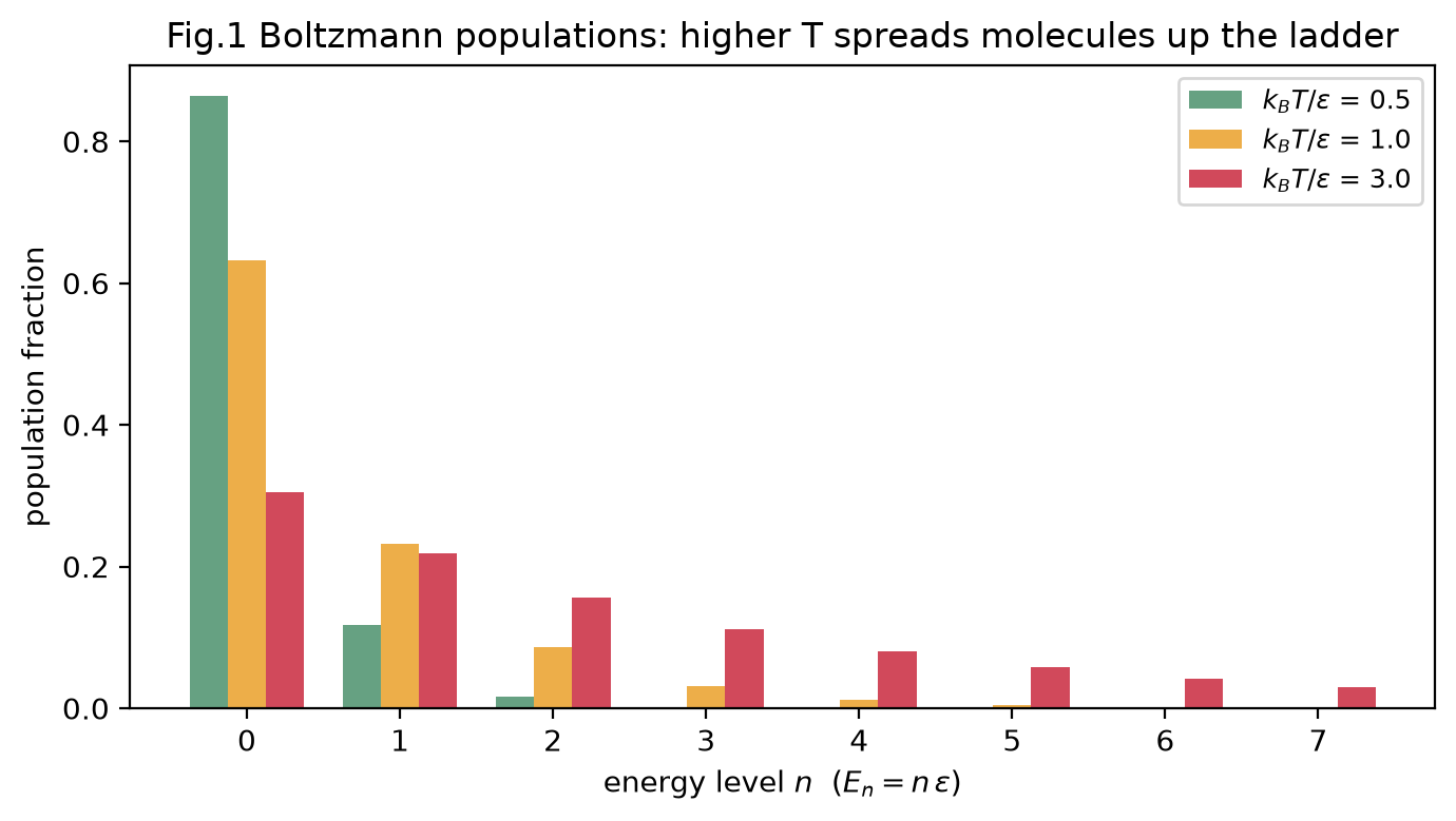

This is the classical statistical backdrop. Quantum mechanics keeps the Boltzmann factor intact but insists the energies $E_i$ are the discrete eigenvalues of $\hat H$ , which is why populations are the bridge from quantized levels to measurable intensities.

Blackbody radiation: where classical physics fails¶

A blackbody is an ideal object that absorbs and re-emits all radiation. The light inside a heated cavity is a gas of electromagnetic standing waves, and classical physics tries to predict how its energy is distributed over wavelength.

Counting the standing-wave modes and giving each the equipartition energy $k_BT$ gives the Rayleigh-Jeans law. It works at long wavelengths but is a disaster at short ones: the number of modes grows without bound, so the predicted energy density diverges as $\lambda\to 0$ . This is the ultraviolet catastrophe, and it says a warm object should glow infinitely bright in the ultraviolet, which is absurd.

Planck’s fix was radical: an oscillator of frequency $\nu$ cannot take just any energy, only integer multiples $E_n = nh\nu$ . With quantized energies, the average energy of a mode is no longer $k_BT$ but

\langle E \rangle = \frac{h\nu}{e^{h\nu/k_BT} - 1},

(4)

which equals $k_BT$ when $h\nu \ll k_BT$ (recovering the classical result) but falls to zero when $h\nu \gg k_BT$ . High-frequency modes are frozen out because one quantum $h\nu$ costs more than the thermal energy available. This gives the Planck radiation law:

import numpy as np
import matplotlib.pyplot as plt

h, c, kB = 6.626e-34, 3.0e8, 1.381e-23
lam = np.linspace(100e-9, 3000e-9, 400)   # 100 nm to 3000 nm

def planck(lam, T):
    return (8 * np.pi * h * c / lam**5) / (np.exp(h * c / (lam * kB * T)) - 1)

def rayleigh_jeans(lam, T):
    return 8 * np.pi * kB * T / lam**4

fig, axes = plt.subplots(1, 2, figsize=(11, 4.2))

# Panel a: Planck curves shift and grow with temperature
for T, col in zip([3000, 4000, 5000], ['#66a182', '#edae49', '#d1495b']):
    axes[0].plot(lam * 1e9, planck(lam, T), color=col, lw=2, label=f'{T} K')
axes[0].set_xlabel('wavelength (nm)')
axes[0].set_ylabel('energy density')
axes[0].legend(fontsize=9)
axes[0].set_title('Fig.2a Planck spectrum shifts to shorter wavelength as T rises')

# Panel b: the ultraviolet catastrophe at one temperature
T = 4000
axes[1].plot(lam * 1e9, planck(lam, T), color='#2e4057', lw=2, label='Planck (quantized)')
axes[1].plot(lam * 1e9, rayleigh_jeans(lam, T), '--', color='#d1495b', lw=2,
             label='Rayleigh-Jeans (classical)')
axes[1].set_ylim(0, 1.2 * planck(lam, T).max())
axes[1].set_xlabel('wavelength (nm)')
axes[1].set_ylabel('energy density')
axes[1].legend(fontsize=9)
axes[1].set_title('Fig.2b Classical theory diverges at short wavelength (UV catastrophe)')

plt.tight_layout()
plt.show()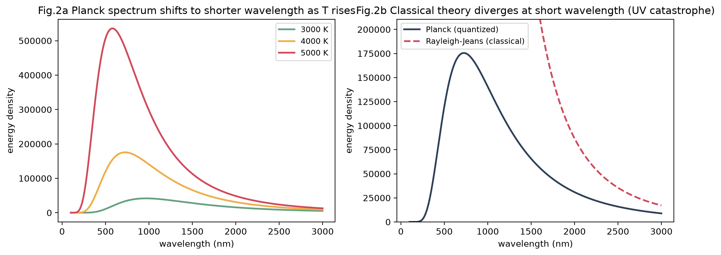

The dashed classical curve shoots up toward short wavelengths while the real spectrum (and Planck’s formula) turns over and falls. Matching the data required quantized energy, and the constant Planck introduced to make it work, $h$ , is the same one at the center of the whole course. Blackbody radiation is where quantization was first forced on physics, and it is the opening story of Chapter 1.

Populations and spectroscopy¶

The Boltzmann distribution is not just background; it sets what you actually see in a spectrum. A molecule can only absorb light from a level it currently occupies, so the intensity of a spectral line is proportional to the population of its starting level. Two consequences run through Chapters 4 through 6:

Vibrations. Vibrational spacings are large compared with $k_BT$ at room temperature, so almost all molecules sit in the ground vibrational state. Infrared absorption therefore starts overwhelmingly from $v = 0$ .
Rotations. Rotational spacings are small compared with $k_BT$ , so many rotational levels are populated. The intensity envelope of a rotational spectrum traces the Boltzmann population across the levels, peaking at an intermediate $J$ and then falling.

So the same $e^{-E/k_BT}$ factor that governs blackbody modes governs the brightness of every line in a molecular spectrum. Quantized energies come from solving the Schrodinger equation; how strongly each level shows up comes from statistics.

Problems¶

Problem 1: Equipartition energy of a gas¶

Using equipartition, find the average translational kinetic energy of one argon atom at $T = 300\ \text{K}$ .

Solution

Three translational degrees of freedom give

\langle E\rangle = \tfrac{3}{2}k_BT = \tfrac{3}{2}(1.381\times10^{-23})(300) \approx 6.2\times10^{-21}\ \text{J}.

(6)

Problem 2: Population ratio¶

Two levels are separated by $\Delta E = k_BT$ . What fraction of the molecules in the upper level relative to the lower?

Solution

\frac{P_2}{P_1} = e^{-\Delta E/k_BT} = e^{-1} \approx 0.37.

(7)

About 37 percent as many molecules occupy the upper level.

Problem 3: When does classical equipartition hold?¶

Explain, using $\langle E\rangle = h\nu/(e^{h\nu/k_BT}-1)$ , why low-frequency modes obey equipartition but high-frequency modes do not.

Solution

For $h\nu \ll k_BT$ , expand the exponential: $e^{h\nu/k_BT} - 1 \approx h\nu/k_BT$ , so $\langle E\rangle \approx k_BT$ , the classical result. For $h\nu \gg k_BT$ the denominator is enormous and $\langle E\rangle \to 0$ : a full quantum $h\nu$ costs more than the available thermal energy, so the mode is frozen out.

Problem 4: The ultraviolet catastrophe¶

In one or two sentences, state what the Rayleigh-Jeans law predicts as $\lambda \to 0$ and why it is unphysical.

Solution

Rayleigh-Jeans gives $u \propto 1/\lambda^4$ , which diverges to infinity as $\lambda\to 0$ . That would mean any warm body radiates infinite energy at short wavelengths, which violates both experiment and energy conservation.

Problem 5: Vibrational population¶

A vibration has $h\nu = 5 k_BT$ at room temperature. Estimate the fraction of molecules in the first excited vibrational state, and comment on why IR absorption starts from the ground state.

Problem 6: Partition function of a two-level system¶

Write the partition function $Z$ for a system with levels at 0 and $\epsilon$ , and find the average energy $\langle E\rangle = \epsilon\, e^{-\epsilon/k_BT}/Z$ in the limits $T\to 0$ and $T\to\infty$ .

Problem 7: Wien’s shift¶

From the Planck curves in Fig.2a, the peak wavelength moves as temperature rises. State the direction of the shift and name the chemistry consequence for how hot objects change color from red to blue-white.