Spectroscopy of Atoms
Spectroscopy is the study of the interaction between matter and electromagnetic radiation.
By analyzing the emitted or absorbed light, spectroscopy reveals information about the structure and composition of atoms and molecules.
When heated or subjected to electrical discharge, atoms emit radiation at characteristic frequencies. The resulting spectrum is unique for each element, serving as a kind of atomic fingerprint.
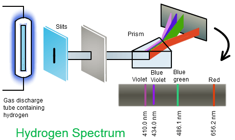
Figure 1:Atomic spectroscopy of the hydrogen atom.
Hydrogen in a gas-discharge tube emits light at discrete wavelengths, which appear as distinct spectral lines when passed through a prism.
Every element produces its own set of lines. Below is what a spectrograph records from a discharge lamp of each gas: no two patterns are alike, which is why a spectrum taken through a telescope tells you what a star is made of.
Source
import numpy as np
import matplotlib.pyplot as plt

def wl_to_rgb(wl):
    """Approximate sRGB colour of a single wavelength in nm."""
    if wl < 440:    r, g, b = -(wl - 440) / 60, 0.0, 1.0
    elif wl < 490:  r, g, b = 0.0, (wl - 440) / 50, 1.0
    elif wl < 510:  r, g, b = 0.0, 1.0, -(wl - 510) / 20
    elif wl < 580:  r, g, b = (wl - 510) / 70, 1.0, 0.0
    elif wl < 645:  r, g, b = 1.0, -(wl - 645) / 65, 0.0
    else:           r, g, b = 1.0, 0.0, 0.0
    return (min(r, 1.0), min(g, 1.0), min(b, 1.0))

# (wavelength in nm, relative brightness) for the strong visible lines
spectra = {
    "H":  [(656.3, 1.0), (486.1, 0.6), (434.0, 0.4), (410.2, 0.3)],
    "He": [(447.1, 0.5), (471.3, 0.3), (492.2, 0.3), (501.6, 0.6),
           (587.6, 1.0), (667.8, 0.5), (706.5, 0.4)],
    "Na": [(498.3, 0.2), (568.8, 0.3), (589.0, 1.0), (589.6, 1.0), (615.4, 0.3)],
    "Hg": [(404.7, 0.6), (435.8, 1.0), (546.1, 1.0), (577.0, 0.6), (579.1, 0.6)],
    "Ne": [(585.2, 0.8), (588.2, 0.6), (594.5, 0.7), (607.4, 0.5), (614.3, 0.7),
           (621.7, 0.5), (626.6, 0.6), (633.4, 0.8), (640.2, 1.0), (650.7, 0.6),
           (659.9, 0.5), (692.9, 0.4), (703.2, 0.5)],
}

fig, axes = plt.subplots(len(spectra), 1, figsize=(9, 4.0), sharex=True)
for ax, (name, lines) in zip(axes, spectra.items()):
    ax.set_facecolor("black")
    for wl, intensity in lines:
        ax.axvline(wl, color=wl_to_rgb(wl), lw=1.8, alpha=0.35 + 0.65 * intensity)
    ax.set_yticks([])
    ax.set_ylabel(name, rotation=0, ha="right", va="center", fontsize=12, labelpad=14)
    for spine in ax.spines.values():
        spine.set_visible(False)
axes[-1].set_xlim(380, 750)
axes[-1].set_xlabel("wavelength (nm)")
fig.suptitle("Fig. Visible emission lines of five elements. Each element has its own fingerprint.",
             fontsize=10)
fig.tight_layout()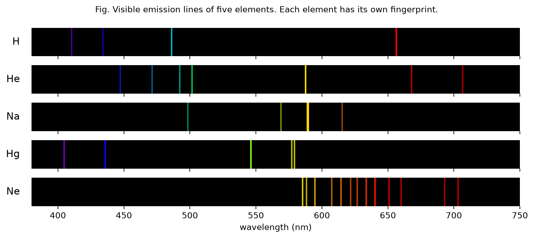
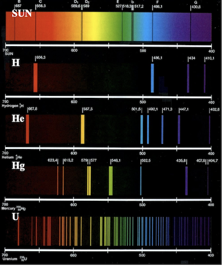
Figure 2:Spectroscopy of the Sun.
By analyzing spectral lines, one can identify the presence of different elements in the solar atmosphere.
Spectral lines and Rydberg’s formula
The existence of discrete spectral lines is impossible to describe with classical mechanics. In 1885, Johann Balmer demonstrated that a subset of the hydrogen atom spectrum (the Balmer series) could be described by the equation
where . Written in terms of the wavenumber this is with . Later, Johannes Rydberg generalized this formula to account for the entire hydrogen atom spectrum yielding the Rydberg formula
While these equations fit the hydrogen atom spectrum nicely, they do not prescribe any physics to the system. They do not present a model of the hydrogen atom but rather a heuristic equation that fits the data. Nonetheless, scientists were perplexed by the presence of the integers and .
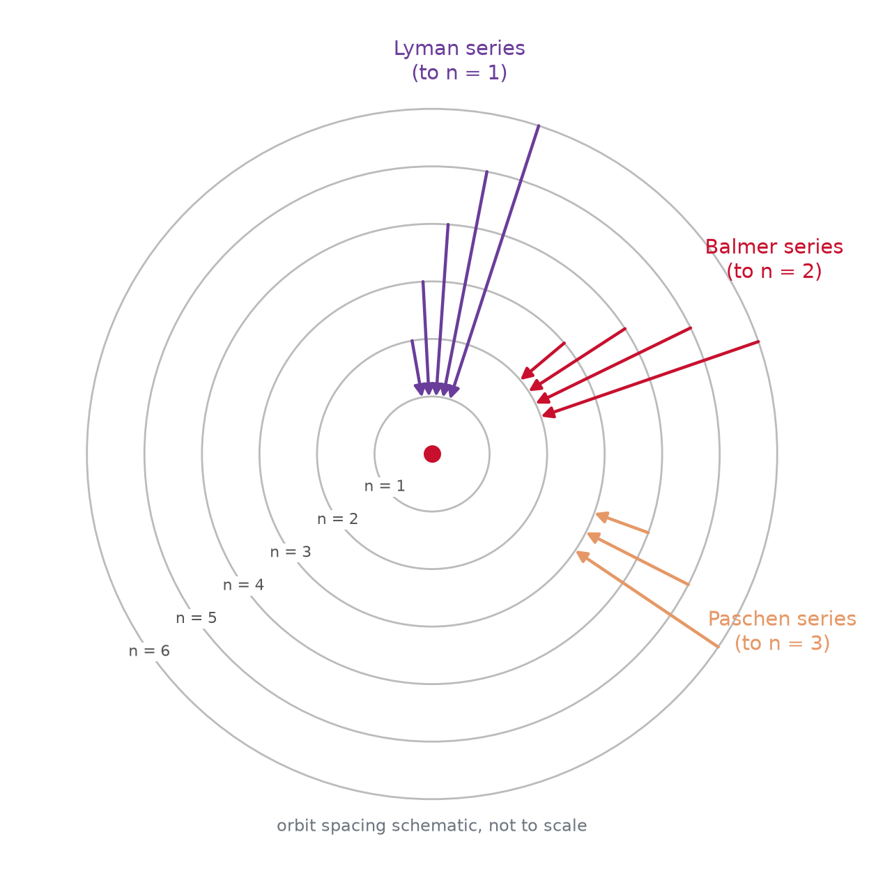
Figure 3:Atomic spectral lines are named after their discoverers. Each series contains all transitions to a distinct lower level .
Bohr’s Model of the Hydrogen Atom
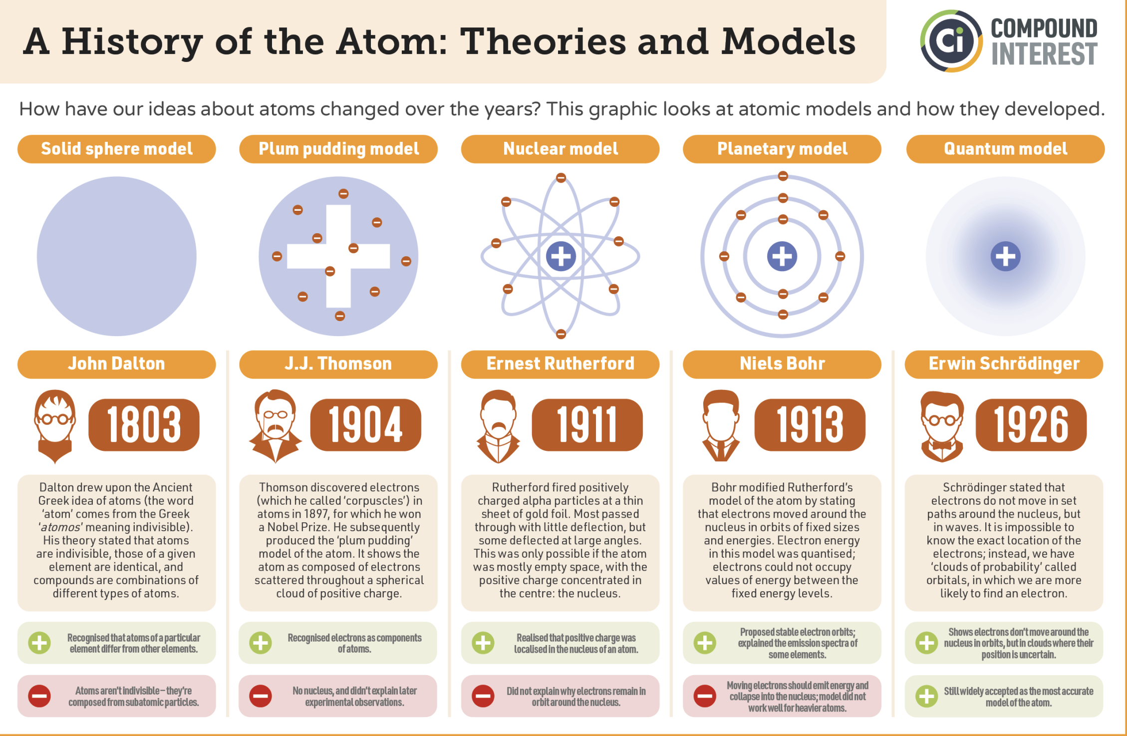
Figure 4:Evolution of atomic models.
From pre-quantum pictures of atoms to the modern quantum mechanical description.
In 1913, Niels Bohr proposed a model of the hydrogen atom that successfully explained its discrete emission spectrum.
The atom was pictured as an electron moving in circular orbits around a central proton. Because the proton is far more massive than the electron, it was treated as fixed in space.
To prevent the electron from spiraling into the nucleus, Bohr introduced a new quantization rule: the electron’s orbital motion must accommodate an integer number of standing wave modes,
This postulate leads directly to an expression for the allowed energy levels of hydrogen, each labeled by a principal quantum number .
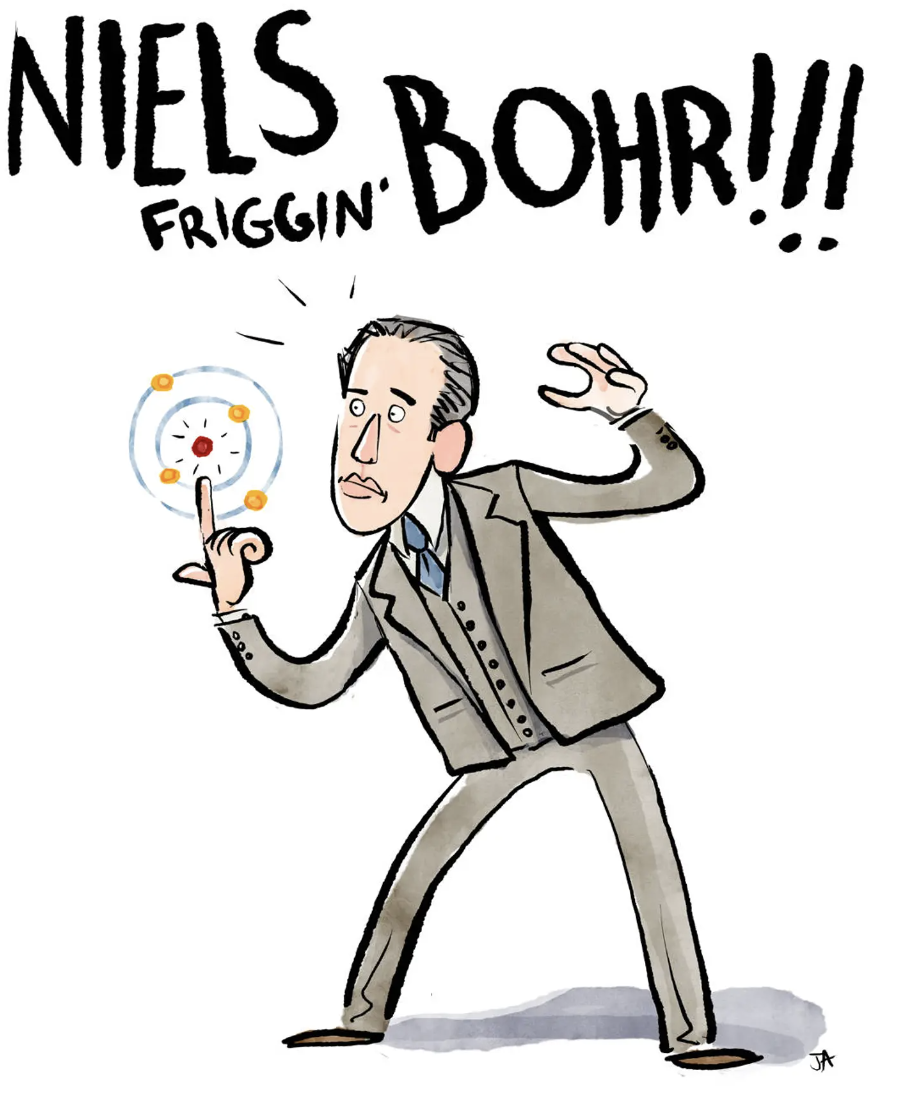
Figure 5:Anecdote about Niels Bohr.
A visitor once noticed a horseshoe (a Scandinavian good-luck charm) hanging above Bohr’s door:
“But Niels, you are a scientist! Surely you don’t believe in this superstition?”
“Of course I don’t,” Bohr replied. “But I am told it works even if you don’t believe in it!”
Quantizing the States of the Electron in the Hydrogen Atom
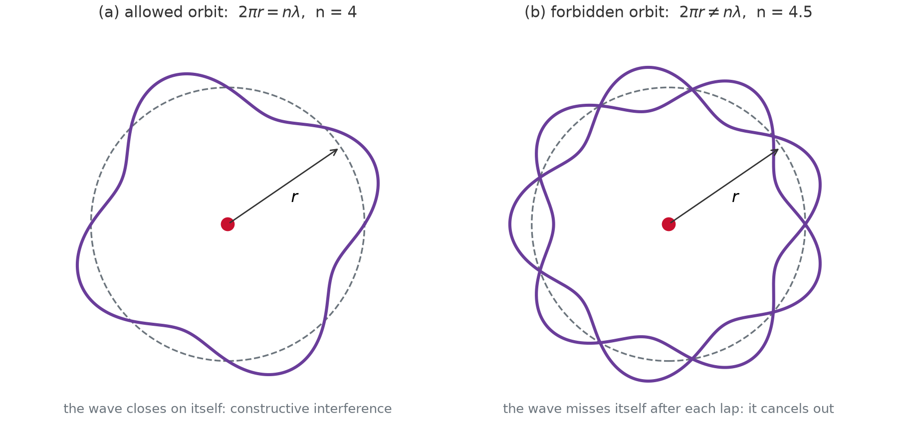
Figure 6:Bohr rationalized discrete orbits by requiring that an integer number of electron wavelengths fit around the circumference of each orbit: four waves close on themselves (a), four and a half do not (b).
Imposing this condition gives the relation
Here, is the de Broglie wavelength of the electron:
Substituting this expression for into the quantization condition yields
We introduce the shorthand because it appears frequently in quantum mechanics. The left-hand side, , represents the angular momentum of the electron.
Thus, Bohr’s model predicts that the electron’s angular momentum is quantized in integer multiples of .
Force Balance
After introducing his quantization rule, Bohr turned back to classical mechanics to determine the allowed electron energies. He assumed that, in a stationary orbit, the electrostatic attraction between the proton and electron is exactly balanced by the centrifugal force of the orbiting electron.
Electrostatic force
where is the elementary charge and the factor ensures SI units.
Centrifugal force
where is the electron mass and its orbital velocity.
Equating these two forces gives
Watch it move: position, velocity and acceleration on a circular orbit
The three vectors keep constant length and only turn. The velocity is always tangent, the acceleration always points at the nucleus, and the centrifugal arrow is its mirror image in the rotating frame. The right panel is worth remembering for later: each component of circular motion is simple harmonic motion, with a quarter cycle ahead of and exactly opposite to it. The same machinery returns for angular momentum in Chapter 4 and the rigid rotor in Chapter 5.
Source
import numpy as np
import matplotlib.pyplot as plt
from matplotlib.animation import FuncAnimation
from matplotlib.patches import Circle
from IPython.display import HTML

TEAL, CARDINAL, GRAY, PURPLE = "#107895", "#C8102E", "#6c757d", "#6a3d9a"
R2, N_FR, OM = 1.0, 72, 1.0           # radius, frames, angular velocity
SV, SA = 0.62, 0.48                   # arrow scale factors
th_seq = np.linspace(0, 2 * np.pi, N_FR, endpoint=False)

fig_cm, (cx, dx) = plt.subplots(1, 2, figsize=(10.4, 4.5),
                                gridspec_kw={"width_ratios": [1.15, 1.2]})

cx.add_patch(Circle((0, 0), R2, fill=False, color=GRAY, lw=1.2, ls="--"))
cx.plot(0, 0, "o", color=CARDINAL, ms=11)
cx.text(0.10, -0.22, "nucleus", color=CARDINAL, fontsize=8)
(bead,) = cx.plot([], [], "o", color="k", ms=9, zorder=6)

def arrow(color, ls="-", lw=2.2):
    return cx.annotate("", xy=(0, 0), xytext=(0, 0), zorder=5,
                       arrowprops=dict(arrowstyle="-|>", color=color, lw=lw,
                                       ls=ls, shrinkA=0, shrinkB=0))

a_r, a_v, a_a, a_cf = arrow(GRAY, lw=1.3), arrow(TEAL), arrow(PURPLE), arrow(CARDINAL, "--")
a_r.arrow_patch.set_alpha(0.45)
cx.set_xlim(-1.75, 1.75)
cx.set_ylim(-1.6, 1.6)
cx.set_aspect("equal")
cx.axis("off")
cx.legend(handles=[plt.Line2D([], [], color=GRAY, lw=1.3, alpha=0.45, label=r"$\vec{r}$  position"),
                   plt.Line2D([], [], color=TEAL, lw=2.2, label=r"$\vec{v}$  velocity (tangent)"),
                   plt.Line2D([], [], color=PURPLE, lw=2.2, label=r"$\vec{a}$  centripetal (inward)"),
                   plt.Line2D([], [], color=CARDINAL, lw=2.2, ls="--",
                              label="centrifugal (rotating frame)")],
          loc="lower center", bbox_to_anchor=(0.5, -0.16), fontsize=7.5, frameon=False)

t_full = th_seq / OM
dx.plot(t_full, R2 * np.cos(th_seq), color=GRAY, lw=1.6, label=r"$x = R\cos\omega t$")
dx.plot(t_full, -OM * R2 * np.sin(th_seq), color=TEAL, lw=1.6, label=r"$v_x = -\omega R\sin\omega t$")
dx.plot(t_full, -OM**2 * R2 * np.cos(th_seq), color=PURPLE, lw=1.6,
        label=r"$a_x = -\omega^2 R\cos\omega t$")
sweep = dx.axvline(0, color="k", lw=0.9, alpha=0.45)
(m_x,) = dx.plot([], [], "o", color=GRAY, ms=7)
(m_v,) = dx.plot([], [], "o", color=TEAL, ms=7)
(m_a,) = dx.plot([], [], "o", color=PURPLE, ms=7)
dx.axhline(0, color="k", lw=0.6, alpha=0.3)
dx.set_xlim(0, t_full[-1])
dx.set_ylim(-1.5, 1.9)
dx.set_xlabel("time")
dx.set_yticks([])
dx.legend(loc="upper right", fontsize=7.5, frameon=False)
dx.set_title("each component is simple harmonic motion", fontsize=9)
for sp in ("top", "right", "left"):
    dx.spines[sp].set_visible(False)

fig_cm.suptitle("Fig. Circular motion: position, velocity and centripetal acceleration.\n"
                "The magnitudes never change, only the directions.", fontsize=10)
fig_cm.tight_layout()

def frame_cm(i):
    th = th_seq[i]
    p = np.array([R2 * np.cos(th), R2 * np.sin(th)])
    rhat, that = p / R2, np.array([-np.sin(th), np.cos(th)])
    bead.set_data([p[0]], [p[1]])
    a_r.xy = p
    a_r.set_position((0, 0))
    a_v.xy = p + SV * OM * R2 * that
    a_v.set_position(p)
    a_a.xy = p - SA * OM**2 * R2 * rhat
    a_a.set_position(p)
    a_cf.xy = p + SA * OM**2 * R2 * rhat
    a_cf.set_position(p)
    sweep.set_xdata([t_full[i], t_full[i]])
    m_x.set_data([t_full[i]], [p[0]])
    m_v.set_data([t_full[i]], [-OM * R2 * np.sin(th)])
    m_a.set_data([t_full[i]], [-OM**2 * R2 * np.cos(th)])
    return bead, a_r, a_v, a_a, a_cf, sweep, m_x, m_v, m_a

ani_cm = FuncAnimation(fig_cm, frame_cm, frames=N_FR, interval=50, blit=False)
plt.close(fig_cm)
HTML(ani_cm.to_jshtml())The force-balance equation together with the quantized angular momentum condition restricts the allowed radii of electron orbits. Solving step by step:
From angular momentum quantization:
Substituting into the force-balance equation:
Simplifying:
Solving for :
where the constant is the Bohr radius, corresponding to the size of the ground-state orbit.
We see clearly that the radius of an orbit grows with increasing quantum number .
Energy of the Hydrogen Atom
The total energy of the electron-proton system is the sum of the electron’s kinetic energy and the Coulomb potential energy:
Using the force-balance relation
we substitute into the energy expression:
Next, inserting the quantized orbital radius
gives the Bohr energy levels:
Spectral lines and the Rydberg constant
The energy difference between two levels and is
Relating this to photon energy and the wavenumber gives
where is the Rydberg constant, which we now know expressed in fundamental constants rather than obtained as the result of an experimental fit!
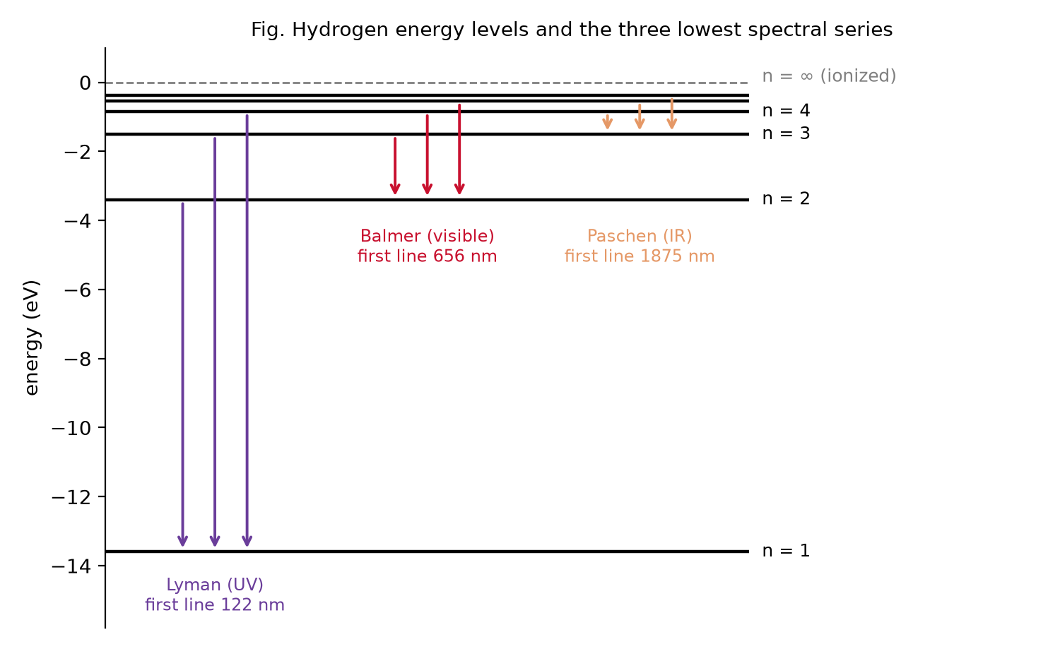
Figure 7:Fig. Hydrogen energy levels and the three lowest spectral series. Every series shares one lower level, and the lines of a series crowd together as grows, converging on the series limit where the electron is set free.
Hydrogen-like atoms
For one-electron atoms such as and , the Bohr model still works, but we have to account for the increased nuclear charge .
E.g. for the atom , for , etc.
Explore the hydrogen spectrum
Every spectral series is the set of transitions that end on one lower level. Slide to move from the Lyman series (ultraviolet) through Balmer (the visible lines of a hydrogen lamp) to Paschen and Brackett (infrared). Raise to see how a one-electron ion like pulls all levels down by and pushes every line to shorter wavelengths.
Where Bohr’s model breaks down
Bohr’s model reproduces the hydrogen spectrum to four digits, and that success is exactly why its failures matter. Within a decade it was clear that the model was a lucky halfway house rather than the final theory.
It fails for every atom with more than one electron. Applied to neutral helium it misses the measured ionization energy of 24.6 eV badly, and it says nothing at all about the periodic table.
It predicts where lines are but not how bright. Real spectra have strong lines, weak lines, and transitions that never appear at all. Bohr’s rules give no intensities and no selection rules.
It cannot see fine structure. At high resolution each Balmer line splits into closely spaced components, and a magnetic field splits them further (the Zeeman effect). A single quantum number has no room for this.
It assumes an orbit at all. A definite radius together with a definite speed violates the uncertainty principle from the previous lecture. The ground state of hydrogen in fact has zero orbital angular momentum, not .
What survives is the physics, not the picture: energies are quantized, the quantum number is an integer, and light is emitted when the atom drops from one level to another. Chapter 5 replaces the orbit with a wavefunction and gets the levels right for the right reason, Chapter 6 supplies the missing selection rules, and Chapter 7 takes on helium.
Problems
Problem 1: Lyman alpha
The so-called Lyman series of lines in the emission spectrum of hydrogen corresponds to transitions from various excited states to the n = 1 orbit. Calculate the wavelength of the lowest-energy line in the Lyman series to three significant figures. In what region of the electromagnetic spectrum does it occur?
Solution
A We can use the Rydberg equation to calculate the wavelength for the Lyman series, .
The lowest energy results from a transition to or from the nearest energy level, hence .
Spectroscopists often talk about energy and frequency as equivalent. The unit (wavenumbers) is particularly convenient. We can convert the answer in part A to
and
This emission line is called Lyman alpha. It is the strongest atomic emission line from the Sun and drives the chemistry of the upper atmosphere of all the planets, producing ions by stripping electrons from atoms and molecules. It is completely absorbed by oxygen in the upper stratosphere, dissociating O2 molecules into O atoms, which react with other O2 molecules to form stratospheric ozone.
B This wavelength is in the UV region of the spectrum.
Problem 2: Photon from n = 4 to n = 1
A. Calculate the energy of a photon that is produced when an electron in a hydrogen atom goes from an orbit with to an orbit with .
B. What happens to the energy of the photon as the initial value of approaches infinity?
Solution
A. We will use Bohr’s formula in electron volts, , to calculate the energy of a photon.
B. The energy of the photon goes up as the electron starts from higher and higher levels, but it saturates. As the photon energy approaches the ionization energy of hydrogen: . Lines pile up against this limit, which is why each spectral series ends in a continuum.
Problem 3: First lines of the Lyman series
Use Rydberg’s formula to calculate the first few lines of the Lyman series ().
Solution
Problem 4: Which level did the electron come from?
A line in the Lyman series of hydrogen has a wavelength of . Find the original level of the electron.
Solution
We are given a wavelength and asked to find the original level of the electron in the Lyman series (where ).
Using the Rydberg formula:
For the Lyman series, , so the equation becomes:
Rearranging to solve for :
Substituting the values:
Now, solving for :
Since must be an integer, we round it to .
Thus, the original level of the electron is .
Problem 5: Ionization energy of He+
Using Bohr theory calculate the ionization energy of singly ionized helium .
Solution
The ionization energy is the energy required to remove an electron from its ground state to infinity. Using Bohr’s theory, the energy of an electron in an orbit is given by:
Where:
is the atomic number,
is the Rydberg energy, the ionization energy of hydrogen (not to be confused with the Rydberg constant in , which is ),
is the principal quantum number.
For singly ionized helium , the atomic number . In the ground state, .
Thus, the energy in the ground state is:
The ionization energy is the negative of this ground state energy (since we want to bring the electron to ):
Therefore, the ionization energy of singly ionized helium is .
Problem 6: Bohr radii
Calculate the radii of the Bohr orbits for the first few levels.
(Optional) Using python plot vs
Solution
The radius of the Bohr orbit is given by the formula:
Where:
is the principal quantum number (level),
is the Bohr radius for hydrogen,
is the atomic number (for hydrogen, ).
For hydrogen (), the radii for the first few levels are:
For :
For :
For :
For :
Therefore, the radii of the Bohr orbits for the first few levels are:
,
,
,
.
Problem 7: The color of H-alpha
The brightest visible line of hydrogen, H-alpha, is the transition of the Balmer series. Compute its wavelength and name its color. Do the same for (H-beta). These two lines are what you see in a hydrogen discharge tube, and they give emission nebulae their red glow.
Problem 8: A coincidence between He+ and H
Show that the transition of emits a photon of exactly the same energy as the (Lyman alpha) transition of hydrogen. Find the general rule: which transitions coincide with hydrogen lines, and why?
Problem 9: How fast is the electron?
Using and , find the speed of the electron in the ground state of hydrogen and express it as a fraction of the speed of light. This dimensionless ratio is the fine-structure constant . What does it say about the need for relativity in hydrogen, and what happens to the innermost electron of uranium ()?
Problem 10: The edge of a series
Every spectral series has a longest wavelength (its first line) and a shortest (the series limit, ). Compute both for the Paschen series (). In which region of the electromagnetic spectrum do they fall, and can the Paschen lines ever overlap with the Balmer lines?