| Property | Linear Momentum | Angular Momentum |
|---|---|---|
| Physical nature | Motion along a straight line | Rotation about an axis |
| Vector form | ||
| Effective mass | ||
| Velocity | ||
| Magnitude (scalar form) | ||
| Kinetic energy | ||
| Quantum operator | ||
| Conservation law | Conserved if no net external force acts | Conserved if no net external torque acts |
| Conservation condition |
velocity vs angular velocity
In circular motion, angular velocity () measures how fast the angle changes, while linear velocity () measures how fast the object moves along the circular path.
For a full rotation, the arc length traveled is related to the angle by
Differentiating with respect to time gives
or equivalently,
Thus, angular velocity is the rate of rotation per unit radius: objects farther from the axis move faster linearly for the same angular speed.
Moment of inertia
Consider a rigid body rotating about a fixed axis with angular velocity . Each particle of mass at distance from the axis moves with linear velocity
The kinetic energy of that particle is
For the whole body, total rotational kinetic energy is the sum over all particles:
We define the term in parentheses as the moment of inertia:
Interpretation
The factor naturally appears from the kinetic energy of rotational motion: it weights each mass element by how far it lies from the axis, determining its contribution to rotational inertia.
Conservation of momentum is due to symmetry
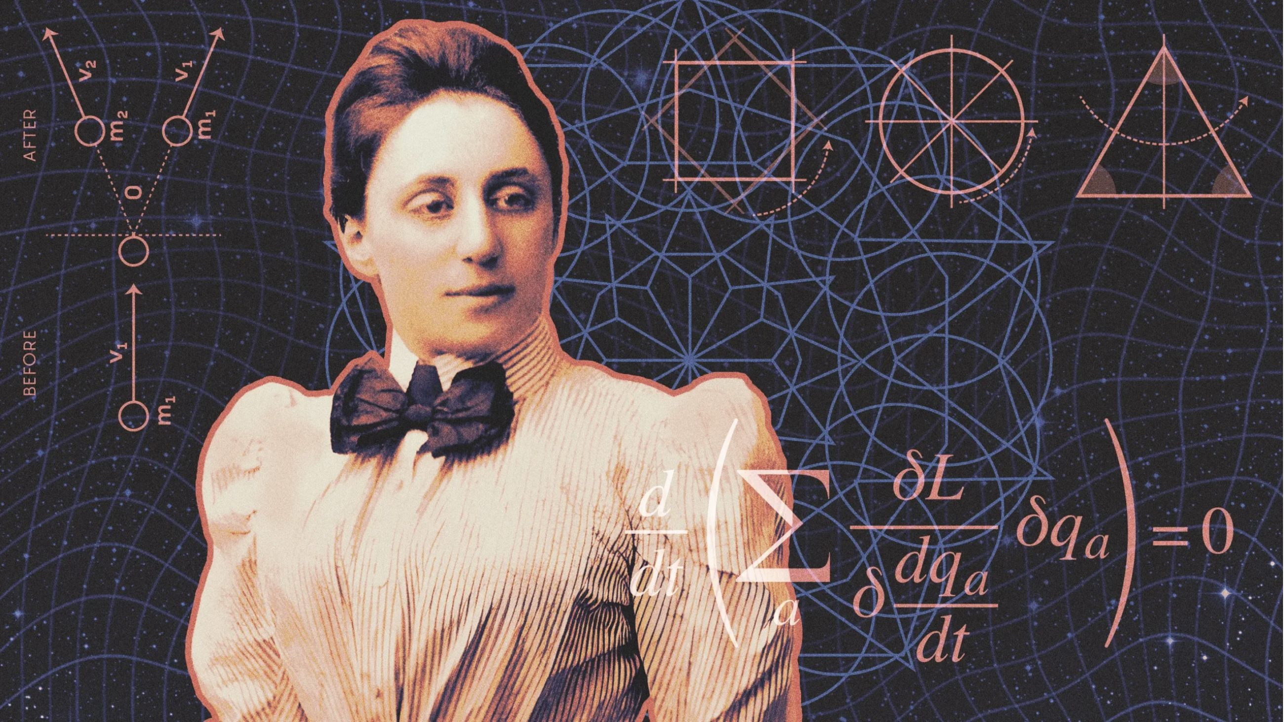
Figure 1:Emmy Noether, a German mathematician whose first and second theorems are fundamental to mathematical physics. See more about her here.
Conservation of momenta
Linear momentum is defined as
From Newton’s second law,
Thus, when no external force acts on a system,
meaning linear momentum is conserved.
Angular momentum is defined as .
Taking the time derivative gives
Therefore, when no external torque acts on the system,
so angular momentum is conserved.
Summary:
No external force → linear momentum conserved.
No external torque → angular momentum conserved.
Classical angular momentum
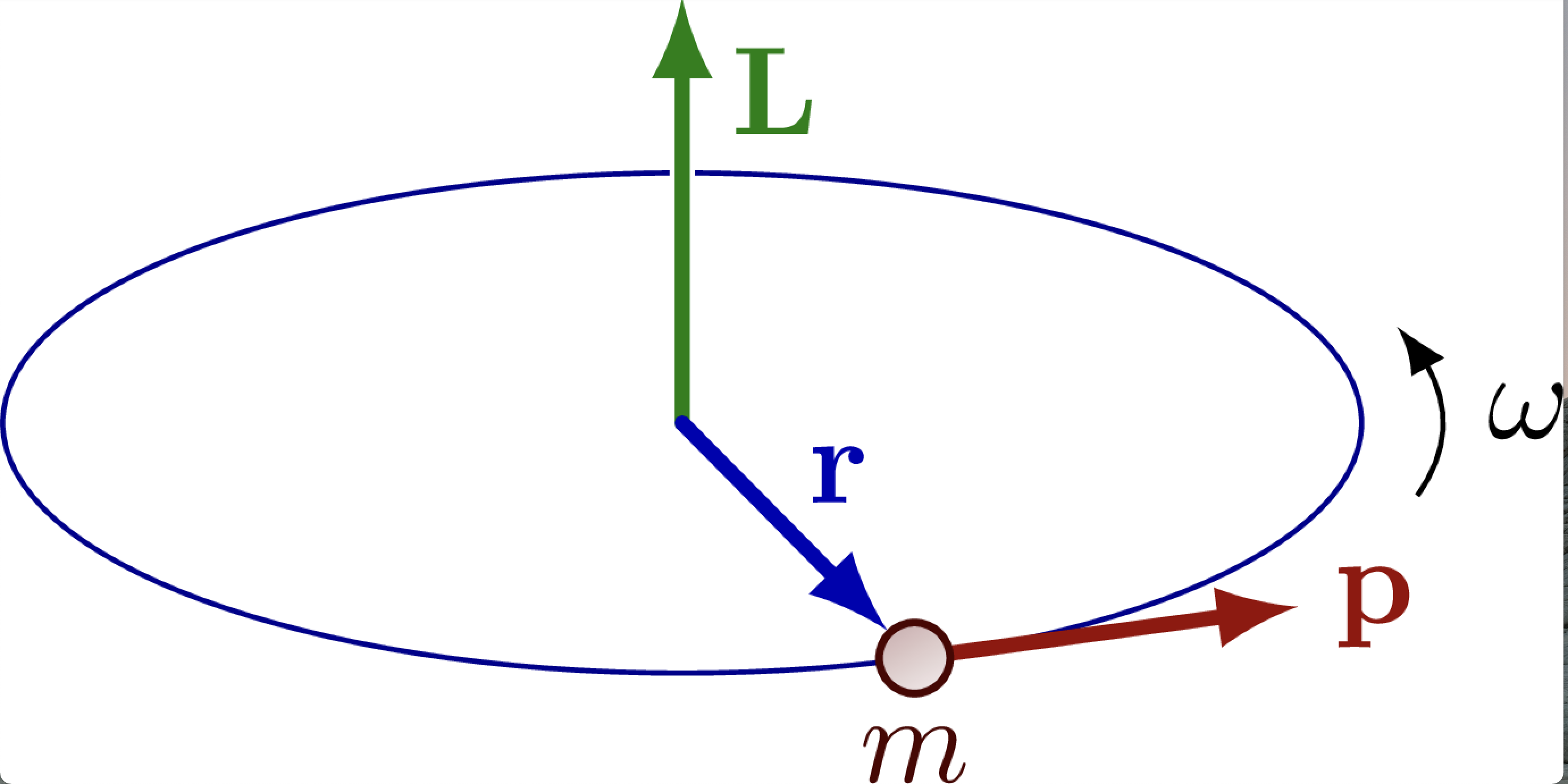
Figure 2:Classical angular momentum, a vector given by the cross product of position and linear momentum. Its direction follows the right-hand rule.
In classical mechanics, the angular momentum is defined via a cross product of position and linear momentum. The cross product is convenient to write using a determinant:
where and denote unit vectors along the and axes. and are components of linear and angular momentum, respectively.
Classical picture: Rotating dumbbell
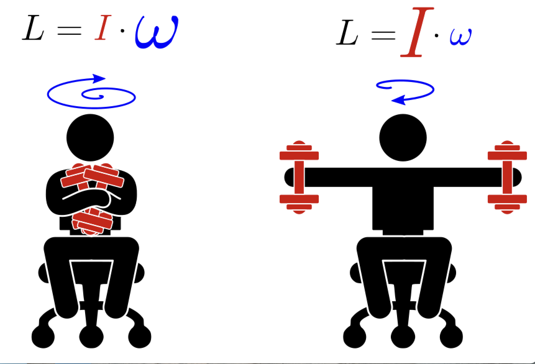
Figure 3:Conservation of angular momentum: with no external torque, total angular momentum stays constant, so lowering the moment of inertia speeds up rotation and raising it slows rotation down.
The rigid rotor is a model of a rotating dumbbell: two unequal masses held together via a rigid stick. The system is not acted upon by any external potential; hence the only energy is the kinetic energy of rotation:
where we have plugged in and , the rotational velocities of the two masses rotating with frequency . The classical mechanical problem of two masses is once again reducible to a single reduced mass rotating at constant radius around the center of mass .
here is the angular momentum, is the moment of inertia, and .
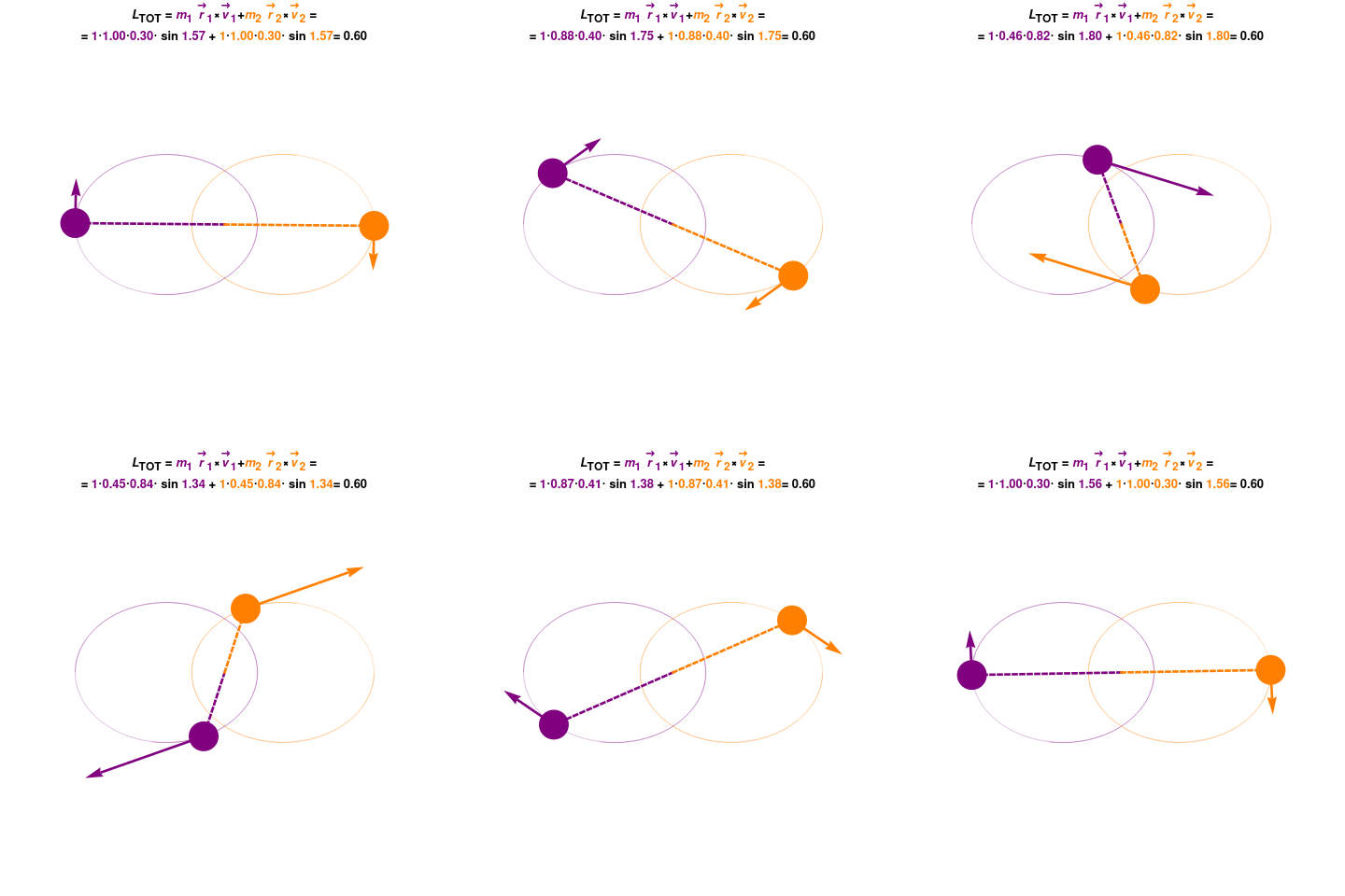
Figure 4:Angular momentum conservation
Spherical coordinates
Spherical coordinates are more convenient for rotational problems where we replace by .
For instance when considering rotation with fixed orbit we are able to eliminate one degree of freedom associated with radial direction.
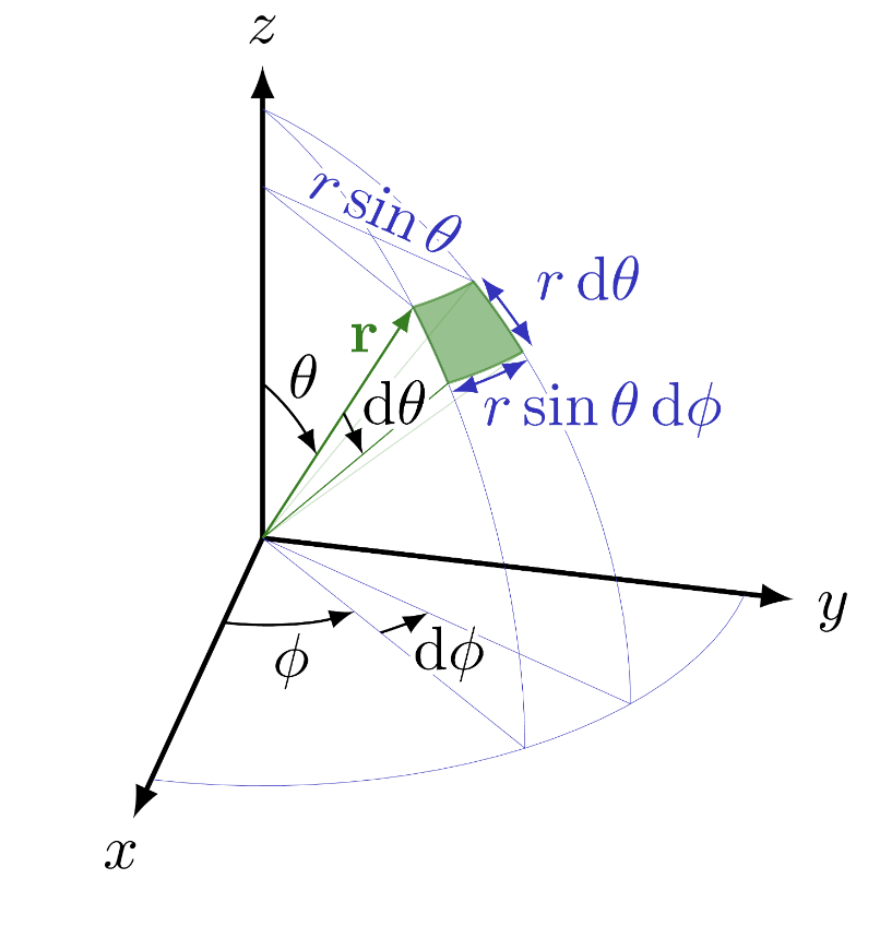
Figure 5:The spherical coordinate system, defined by radial coordinate , azimuthal angle , and polar angle .
Laplacian
Solution
Quantum angular momentum
In quantum mechanics, the classical angular momentum is replaced by the corresponding quantum mechanical operator.
In spherical coordinates, the angular momentum operators can be written in the following form. The derivations are quite tedious, involving multiple applications of the chain rule, but they are just a straightforward mathematical procedure. Note that the choice of -axis here was arbitrary. Sometimes the physical system implies such an axis naturally (for example, the direction of an external magnetic field).
Solution
Components of angular momentum do not commute!
Unlike linear momentum, the components of angular momentum do not commute!
This implies that it is not possible to measure any of the Cartesian angular momentum pairs simultaneously with an infinite precision (the Heisenberg uncertainty relation).
Note the cyclical nature of the commutators between components.
Eigenfunctions and eigenvalues of and 
Since the operators for a component and the angular momentum square commute, it is possible to find functions that are eigenfunctions of both and .
Note that here has nothing to do with magnetism but the name originates from the fact that (electron or nuclear) spins follow the same laws of angular momentum.
describes the projections of on the z axis. E.g., for l=2 there are five projections .
Functions are called spherical harmonics. Examples of spherical harmonics with various values of and are given below (with the Condon-Shortley phase convention).
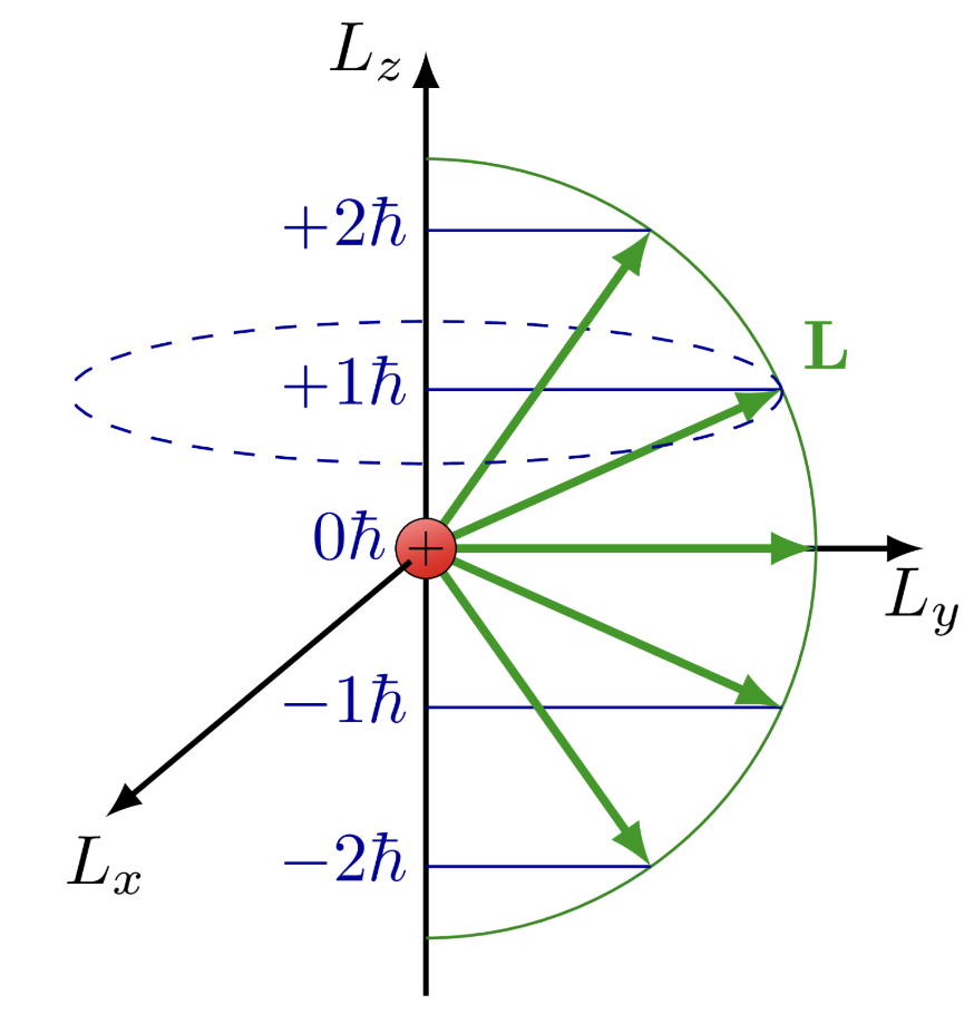
Figure 6:Angular momentum is quantized. Its magnitude can take specific values dictated by . Projections of angular momentum are also quantized and can take specific discrete values dictated by which can take values never exceeding .
Spherical harmonics
Spherical harmonics, denoted as or are important in many theoretical and practical applications, e.g., the representation of multipole electrostatic and electromagnetic fields, computation of atomic orbital electron configurations, representation of gravitational fields, MRI imaging for streamline tractography, and the magnetic fields of planetary bodies and stars.
Spherical harmonics emerge from the angular part of the solutions to the Laplace equation in spherical coordinates, which is the type of equation we obtained for the rigid rotor problem and will see once more in the hydrogen atom problem.
| Expression | Colatitudinal Nodes | Azimuthal Nodes | |
|---|---|---|---|
| 0 | 0 | ||
| 1 (equatorial) | 0 | ||
| 0 | 1 | ||
| 2 (colatitudinal rings) | 0 | ||
| 1 (equatorial) | 1 | ||
| 0 | 2 |
Nodes of Spherical Harmonics
The nodal structure of spherical harmonics is influenced by both the degree and the order , defining the number and type of nodes as follows:
Colatitudinal Nodes (Polar Nodes): The variable defines “polar” nodes, which appear as circular bands around the sphere. The expression in or creates colatitudinal nodes:
For example, with has a single node at , creating an equatorial node.
, with , introduces two polar nodes, dividing the sphere into three regions along the colatitude.
Azimuthal Nodes (Longitudinal Nodes): The variable defines “azimuthal” nodes due to the terms , which create lines of longitude where the function changes phase. The number of azimuthal nodes is determined by :
If , there are no azimuthal nodes, as seen in and .
For , a single azimuthal node occurs (e.g., , ), and for , two azimuthal nodes appear (e.g., ).
Total Nodes: equal to the sum of the polar and longitudinal nodes, and exactly equal to . For instance, has no nodes and has four nodes.
Orthogonality of Spherical Harmonics
The orthogonality of spherical harmonics is expressed as:
This orthogonality condition can be explicitly written as:
Source
import numpy as np
from scipy.special import sph_harm_y
from scipy.integrate import dblquad

def orthogonality_test(l1, m1, l2, m2):
    """
    Computes the orthogonality integral of spherical harmonics Y(l1, m1) and Y(l2, m2).

    Parameters:
    l1, m1 (int): Degree and order of the first spherical harmonic.
    l2, m2 (int): Degree and order of the second spherical harmonic.

    Returns:
    float: The result of the orthogonality integral.
    """
    # Define the integrand for the orthogonality condition
    def integrand(theta, phi):
        Y_lm1 = sph_harm_y(l1, m1, theta, phi)
        Y_lm2 = sph_harm_y(l2, m2, theta, phi)
        return np.real(Y_lm1 * np.conj(Y_lm2)) * np.sin(theta)

    # Perform the integration over theta (0 to pi) and phi (0 to 2*pi)
    integral, error = dblquad(integrand, 0, 2 * np.pi, lambda _: 0, lambda _: np.pi)
    return integral

# Test orthogonality between different spherical harmonics
print("Orthogonality Tests:")
print(f"∫ Y(1,0) * Y(1,0)* = {orthogonality_test(1, 0, 1, 0):.5f} (should be close to 1)")
print(f"∫ Y(1,0) * Y(1,1)* = {orthogonality_test(1, 0, 1, 1):.5f} (should be close to 0)")
print(f"∫ Y(1,1) * Y(2,1)* = {orthogonality_test(1, 1, 2, 1):.5f} (should be close to 0)")
print(f"∫ Y(2,1) * Y(2,1)* = {orthogonality_test(2, 1, 2, 1):.5f} (should be close to 1)")
print(f"∫ Y(2,0) * Y(2,-1)* = {orthogonality_test(2, 0, 2, -1):.5f} (should be close to 0)")
Orthogonality Tests:
∫ Y(1,0) * Y(1,0)* = 1.00000 (should be close to 1)
∫ Y(1,0) * Y(1,1)* = 0.00000 (should be close to 0)
∫ Y(1,1) * Y(2,1)* = 0.00000 (should be close to 0)
∫ Y(2,1) * Y(2,1)* = 1.00000 (should be close to 1)
∫ Y(2,0) * Y(2,-1)* = -0.00000 (should be close to 0)
Plotting Spherical Harmonics
Here we will visualize a spherical harmonic on a 3D sphere of radius 1. The radius is fixed, so there are only two variables that dictate the nodal features:
Colatitudinal nodes depend on and represent bands around the sphere, arising from terms in or .
Azimuthal nodes depend on and create longitudinal nodes based on .
Source
import matplotlib.pyplot as plt
from matplotlib import cm
import numpy as np
from scipy.special import sph_harm_y
from mpl_toolkits.mplot3d import Axes3D

def generate_spherical_harmonic_data(l, m):
    """
    Generates the data needed to plot the spherical harmonic for given l and m values.

    Parameters:
    l (int): Degree of the spherical harmonic.
    m (int): Order of the spherical harmonic.

    Returns:
    tuple: (x, y, z, fcolors_normalized) where:
        - x, y, z are the Cartesian coordinates of the spherical surface,
        - fcolors_normalized is the color data for plotting.
    """

    # Define theta and phi grids
    phi = np.linspace(0, np.pi, 100)          # colatitude
    theta = np.linspace(0, 2 * np.pi, 100)    # azimuth
    phi, theta = np.meshgrid(phi, theta)

    # Cartesian coordinates for the unit sphere
    x = np.sin(phi) * np.cos(theta)
    y = np.sin(phi) * np.sin(theta)
    z = np.cos(phi)

    # Calculate the spherical harmonic Y(l, m) and normalize it to [-1, 1] for color mapping
    fcolors = sph_harm_y(l, m, phi, theta).real
    fcolors_normalized = (fcolors - fcolors.min()) / (fcolors.max() - fcolors.min())

return x, y, z, fcolors_normalizedharmonics
Source
# Define the range of m and l values for the first three spherical harmonics
harmonics = [(0, 1), (1, 1), (-1, 1)]  # List of (m, l) pairs to plot

# Create a figure to hold three subplots in one row
fig = plt.figure(figsize=(18, 6))
fig.suptitle("First Three Spherical Harmonics", fontsize=16)

for i, (m, l) in enumerate(harmonics, start=1):

    x, y, z, fcolors_normalized = generate_spherical_harmonic_data(l, m)

    # Create a subplot for each (m, l) pair in one row
    ax = fig.add_subplot(1, 3, i, projection='3d')
    ax.plot_surface(x, y, z, rstride=1, cstride=1, facecolors=cm.seismic(fcolors_normalized),
                    linewidth=0, antialiased=False)

    # Customize each subplot
    ax.set_title(f"$Y_{{{l},{m}}}$", fontsize=14)
    ax.set_box_aspect([1, 1, 1])  # Ensures spherical aspect ratio
    ax.set_axis_off()             # Turn off axes for clarity

# Adjust layout for a clear view of all subplots in one row
plt.tight_layout(rect=[0, 0, 1, 0.95])
plt.show()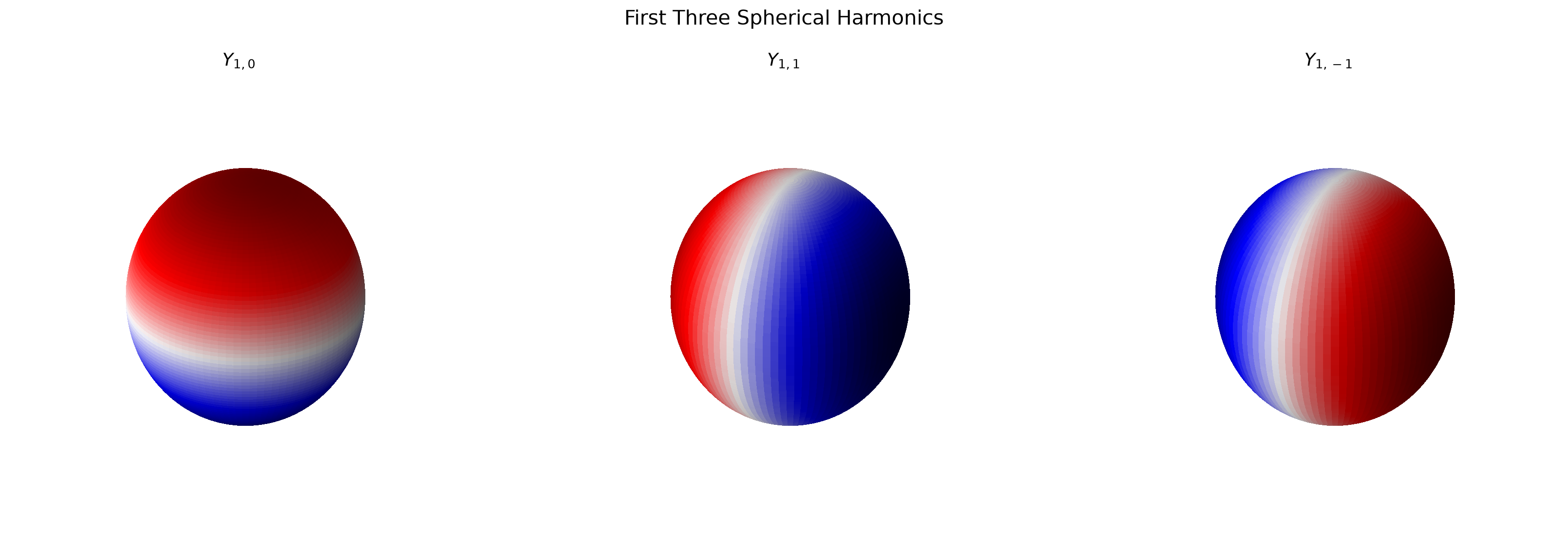
harmonics
Source
import matplotlib.pyplot as plt
from matplotlib import cm
import numpy as np
from scipy.special import sph_harm_y
from mpl_toolkits.mplot3d import Axes3D

# Define l and the range of m values for spherical harmonics with l=2
l = 2
m_values = [-2, -1, 0, 1, 2]

# Create a figure to hold five subplots in a 2x3 layout
fig = plt.figure(figsize=(15, 10))
fig.suptitle("Spherical Harmonics with l=2", fontsize=18)

for i, m in enumerate(m_values, start=1):

    # Calculate the spherical harmonic Y(l, m) and normalize it to [-1, 1] for color mapping
    x, y, z, fcolors_normalized = generate_spherical_harmonic_data(l, m)

    # Create a subplot for each (m, l) pair in a 2x3 grid
    ax = fig.add_subplot(2, 3, i, projection='3d')
    ax.plot_surface(x, y, z, rstride=1, cstride=1, facecolors=cm.seismic(fcolors_normalized),
                    linewidth=0, antialiased=False)

    # Customize each subplot
    ax.set_title(f"$Y_{{2,{m}}}$", fontsize=16)
    ax.set_box_aspect([1, 1, 1])  # Ensures spherical aspect ratio
    ax.set_axis_off()             # Turn off axes for clarity

# Adjust layout for a clear view of all subplots in a 2x3 grid
plt.tight_layout(rect=[0, 0, 1, 0.95])
plt.show()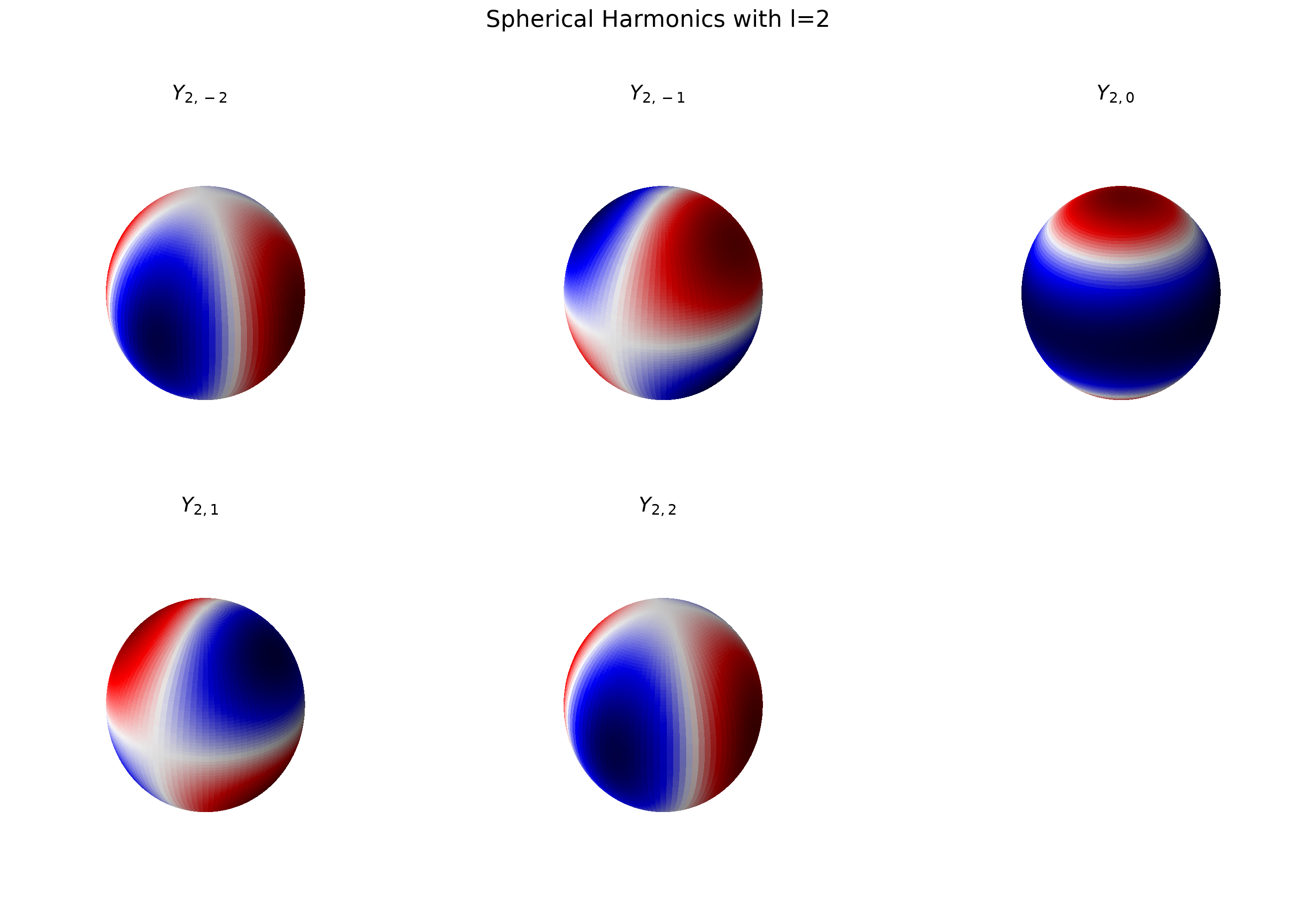
Total number of nodes = 
Source
import plotly.io as pio
pio.renderers.default = "plotly_mimetype"   # interactive in Jupyter-Book
import numpy as np
import plotly.graph_objects as go
from scipy.special import sph_harm_y

# Define the range of m and l values for the first three spherical harmonics
harmonics = [(1, 1), (1, 2), (2, 3)]  # List of (m, l) pairs to plot

# Initialize the figure
fig = go.Figure()


# Loop over each harmonic and create a separate subplot
for i, (m, l) in enumerate(harmonics, start=1):

    # Calculate the spherical harmonic Y(l, m) and normalize it to [0, 1]
    x, y, z, fcolors_normalized = generate_spherical_harmonic_data(l, m)

    # Add the spherical harmonic to the figure as a surface in a new scene
    fig.add_trace(go.Surface(
        x=x, y=y, z=z,
        surfacecolor=fcolors_normalized,
        colorscale='rdbu',
        showscale=False,
        name=f"Y_{{{l},{m}}}",
        scene=f'scene{i}'  # Assign each plot to a different scene
    ))

# Update layout to arrange scenes in a row and add titles as annotations
fig.update_layout(
    title="Three Spherical Harmonics: m=1, l=1, 2, 3",
    scene=dict(domain=dict(x=[0, 0.33]), xaxis=dict(visible=False), yaxis=dict(visible=False), zaxis=dict(visible=False), aspectmode='cube'),
    scene2=dict(domain=dict(x=[0.33, 0.66]), xaxis=dict(visible=False), yaxis=dict(visible=False), zaxis=dict(visible=False), aspectmode='cube'),
    scene3=dict(domain=dict(x=[0.66, 1]), xaxis=dict(visible=False), yaxis=dict(visible=False), zaxis=dict(visible=False), aspectmode='cube'),
    annotations=[
        dict(text="Y_{2,0}", x=0.16, y=1.05, showarrow=False, xref="paper", yref="paper", font=dict(size=14)),
        dict(text="Y_{2,1}", x=0.5, y=1.05, showarrow=False, xref="paper", yref="paper", font=dict(size=14)),
        dict(text="Y_{2,-1}", x=0.83, y=1.05, showarrow=False, xref="paper", yref="paper", font=dict(size=14))
    ]
)

# Display the figure
fig.show()Alternative visualizations of Spherical Harmonics
Before, we visualized spherical harmonics on the unit sphere . However, there are times when we want to visualize how the magnitude of a spherical harmonic changes in space.
For instance, to visualize we could either plot its values on a unit sphere, or we could plot how changes as we move around in space.
Source
import numpy as np
import plotly.graph_objects as go
from plotly.subplots import make_subplots
from scipy.special import sph_harm_y

# Set up the subplots with two side-by-side 3D plots
fig = make_subplots(rows=1, cols=2, specs=[[{'is_3d': True}, {'is_3d': True}]])

# Define theta and phi grids for spherical coordinates
theta = np.linspace(0, np.pi, 100)
phi = np.linspace(0, 2 * np.pi, 100)
theta, phi = np.meshgrid(theta, phi)

# Convert spherical to Cartesian coordinates for the surface plots
x = np.sin(theta) * np.cos(phi)
y = np.sin(theta) * np.sin(phi)
z = np.cos(theta)

# Compute the spherical harmonic Y_{1,-1}
m, l = -1, 1
r0a = np.sqrt(3 / (4 * np.pi)) * y  # Y_{1,-1} harmonic on y-axis
r0 = np.abs(r0a)  # Absolute value for magnitude scaling

# First plot: Scaled by the spherical harmonic (bead-like structure)
fig.add_trace(
    go.Surface(
        x=r0 * x, y=r0 * y, z=r0 * z,  # Scale coordinates by |Y_{1,-1}|
        surfacecolor=r0a,  # Color by Y_{1,-1} values
        colorscale='RdBu'
    ),
    row=1, col=1
)

# Second plot: Standard unit sphere with grayscale color
fig.add_trace(
    go.Surface(
        x=x, y=y, z=z,  # Unit sphere without scaling
        surfacecolor=z,  # Color by z-coordinate for simplicity
        colorscale='RdBu'
    ),
    row=1, col=2
)

# Update layout for both plots
fig.update_layout(
    font_family="JuliaMono",
    showlegend=False,
    margin=dict(l=0, r=0, b=0, t=0),
    paper_bgcolor='rgba(0,0,0,0)',
)

# Set scene properties with adjusted axis limits for each plot
fig.update_scenes(
    dict(
        xaxis=dict(nticks=4, range=[-0.5, 0.5]),  # Limit range to reduce empty space
        yaxis=dict(nticks=4, range=[-0.5, 0.5]),
        zaxis=dict(nticks=4, range=[-0.5, 0.5]),
        aspectratio=dict(x=1, y=1, z=1)
    ),
    row=1, col=1
)
fig.update_scenes(
    dict(
        xaxis=dict(nticks=4, range=[-1.8, 1.8]),
        yaxis=dict(nticks=4, range=[-1.8, 1.8]),
        zaxis=dict(nticks=4, range=[-1.8, 1.8]),
        aspectratio=dict(x=1, y=1, z=1)
    ),
    row=1, col=2
)

# Hide color scales for a cleaner look
fig.update_traces(showscale=False)

# Show the plot
fig.show()Source
import numpy as np
import plotly.graph_objects as go
from plotly.subplots import make_subplots
from matplotlib import cm
import matplotlib
import matplotlib.pyplot as plt

# Define theta (angle) values
theta = np.linspace(0, 2 * np.pi, 100)

# Compute spherical harmonic values (scaled sin(theta) for two-lobe structure)
Y_1m1_values = np.sin(theta)  # Y_{1,-1} varies with sin(theta) for the two-lobe shape
r_values = np.abs(Y_1m1_values)  # Radial scaling based on |Y_{1,-1}|

# Set up the color map
cmap = matplotlib.colormaps["RdBu"]
norm = plt.Normalize(vmin=-1, vmax=1)

# Create subplots for two polar plots
fig = make_subplots(rows=1, cols=2, specs=[[{'type': 'polar'}, {'type': 'polar'}]])

# First polar plot: Two-lobed structure with color gradient
for i in range(len(theta) - 1):
    fig.add_trace(
        go.Scatterpolar(
            r=[r_values[i], r_values[i + 1]],
            theta=[np.degrees(theta[i]), np.degrees(theta[i + 1])],
            mode="lines",
            line=dict(color=matplotlib.colors.to_hex(cmap(norm(Y_1m1_values[i]))), width=5),
            showlegend=False
        ),
        row=1, col=1
    )

# Second polar plot: Unit circle with consistent color gradient
for i in range(len(theta) - 1):
    fig.add_trace(
        go.Scatterpolar(
            r=[1, 1],  # Fixed radius for unit circle
            theta=[np.degrees(theta[i]), np.degrees(theta[i + 1])],
            mode="lines",
            line=dict(color=matplotlib.colors.to_hex(cmap(norm(Y_1m1_values[i]))), width=5),
            showlegend=False
        ),
        row=1, col=2
    )

# Update layout for both polar plots with fixed radius range and equal appearance
fig.update_layout(
    font_family="JuliaMono",
    showlegend=False,
    margin=dict(l=0, r=0, b=0, t=0),
    polar=dict(radialaxis=dict(range=[0, 1.2])),  # First plot axis range
    polar2=dict(radialaxis=dict(range=[0, 1.2]))  # Second plot axis range
)

# Show the plot
fig.show()