Quantum rigid rotor and angular momentum operator
The Hamiltonian for the rigid rotor model is the kinetic energy operator of an effective mass which rotates around a sphere of radius .
To incorporate the constraint it is more convenient to adopt spherical coordinates . The full Laplacian in spherical coordinates is:
In spherical coordinates the Hamiltonian is more conveniently expressed in terms of the angular momentum operator as opposed to the linear momentum operator:
Where is the moment of inertia and we have identified the angular momentum operator as:
Quantum numbers for quantizing coordinate pair.
Having written down the Hamiltonian we now solve it, anticipating two quantum numbers for two coordinates.
The eigenfunctions turn out to be well-known special functions called spherical harmonics :
We are once again able to separate two angular variables and solve the resulting ODE exactly.
We expect the energy to depend on two quantum numbers and , which quantize rotational motion across the and angles.
Rotational states of molecules are quantized
Solving the rigid rotor problem reveals that rotational energy eigenvalues depend only on the quantum number .
Each energy level is therefore -fold degenerate, corresponding to the allowed values of the magnetic quantum number .
The quantization of rotational motion arises from the cyclic boundary condition rather than from any potential energy term (which is zero for a free rotor).
There is no rotational zero-point energy, since the state is allowed.
The ground-state rotational wavefunction corresponds to an isotropic distribution, with equal probability for all orientations.
Solution
First we calculate the reduced mass:
and are given by the eigenvalue expressions of the respective operators:
The energy of the level is given by the eigenvalue expression of the Hamiltonian:
This rotational spacing can be observed, for example, in the gas-phase infrared spectrum of HCl.
Rotational spectra of diatomic molecules
We assume that the molecule is a rigid rotor, which means that the molecular geometry does not change during rotation. We have solved this problem already.
Energies are typically expressed in wavenumber units (, although the basic SI unit is ) by dividing by . The use of wavenumber units is denoted by a tilde above the variable (e.g., ).
Within the rigid rotor approximation we can derive selection rules by computing the transition dipole moment using properties of the spherical harmonics.
Spectral lines and rotational constant determination
When we compute the energy spacing we see that it depends linearly on the quantum level . This means we can take one more difference and easily eliminate it, getting a constant:
The successive line positions in the rotational spectrum are given by . Note that molecules with different atomic isotopes have different moments of inertia and hence different positions for the rotational lines.
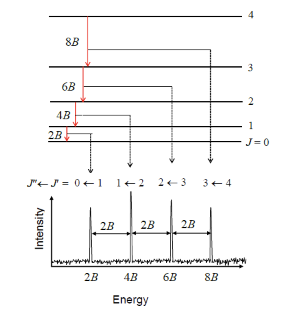
Figure 1:The rigid rotor model predicts evenly spaced spectral lines.
Population of rotational states
Another factor that affects the line intensities in a rotational spectrum is related to the thermal population of the rotational levels. Thermal populations of the rotational levels is given by the Boltzmann distribution (for a collection of molecules):
Here is called the partition function, and is the degeneracy of state . A useful reference for the thermal energy is : if the energy of a state is much higher than this, it will not be thermally populated.
One expects the intensities to first increase as a function of the initial state , reach a maximum, and then decrease as the thermal populations fall off. In an absorption experiment, one can see the thermal populations of the initial rotational levels.
Note: for systems where the rotational degrees of freedom may exchange identical nuclei, an additional complication arises from the symmetry requirement on the nuclear wavefunction. Recall that bosons must have symmetric wavefunctions and fermions antisymmetric ones. We will not discuss this in more detail here.
Solution
The level populations are given by the Boltzmann distribution:
where is the number of molecules in the rotational ground state. First we calculate the factor appearing in the exponent:
Then, for example, for we get:
The same way one can get the relative populations as: 1.00, 2.71, 3.70, 3.84, 3.31, and 2.45 for . Note that these are relative populations since we did not calculate the partition function .
Ro-vibrational spectra, R, P and Q branches
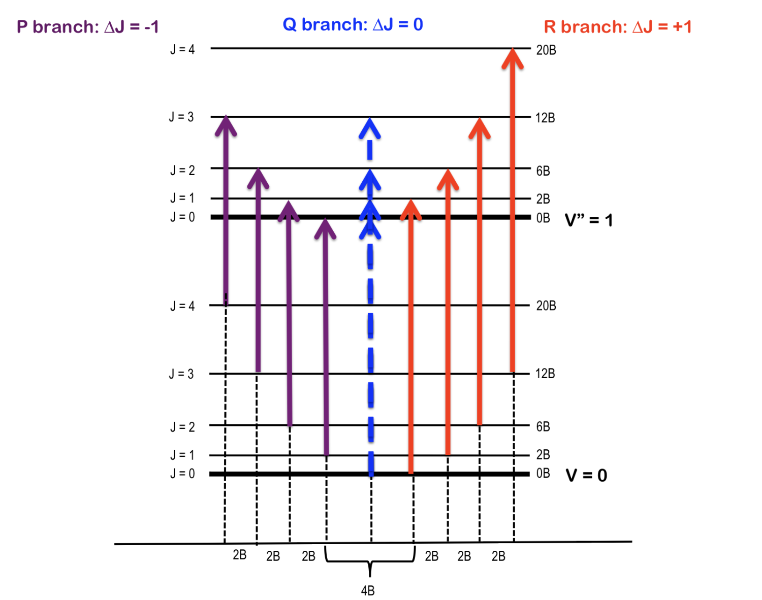
Figure 2:Cartoon of an idealized rovibrational spectrum showing the P, Q, and R branches.
Often we are interested in transitions among rotational levels that accompany excitation from the ground vibrational state, . This can be described by combining the rigid rotor and harmonic oscillator models:
Since at room temperature molecules mostly occupy the vibrational ground state, we are interested in rotational transitions taking place between the ground () and the first excited () vibrational states.
Rigid rotor model predicts different frequencies for absorption and emission transitions between any two rotational states and given by where the refers to the initial rotational state and is the final state.
The transitions with are called R branch:
The transitions with are called P branch:
The Q-branch is predicted to be absent because it is forbidden by the selection rule of the rigid rotor model.
Rigid rotor and real microwave spectra
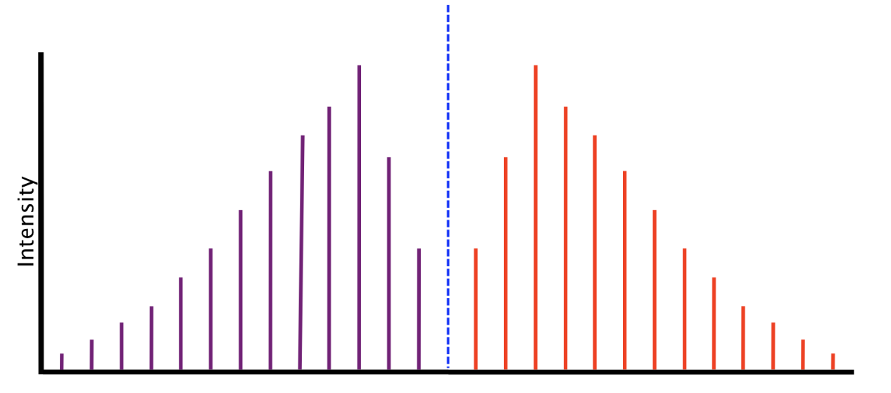
Figure 3:Idealized rovibrational spectrum predicted by the rigid rotor model.
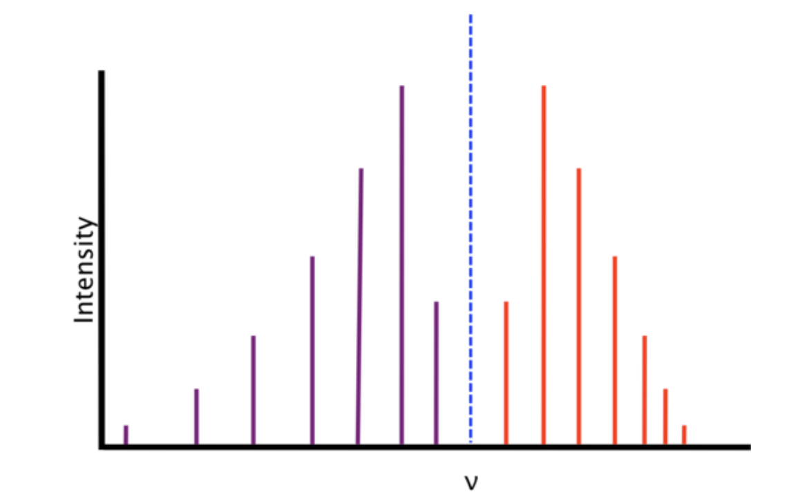
Figure 4:A real rovibrational spectrum, showing departures from the idealized rigid rotor pattern.
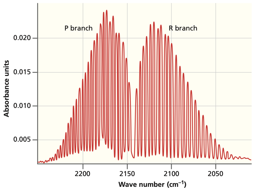
Figure 5:High-resolution spectrum of CO, with the P and R branches resolved into individual rotational transitions.
Rovibronic Coupling
As a diatomic molecule vibrates, its bond length oscillates. Because the moment of inertia depends on the bond length, it also changes during vibration, leading to a variation in the rotational constant .
In earlier approximations, we assumed that the rotational constants of the and transitions were identical. In reality, they differ due to this rovibrational coupling.
The dependence of on the vibrational quantum number can be expressed as:
where is the equilibrium rotational constant (for a rigid rotor), and is the rotation–vibration coupling constant. From observed band spectra, one can determine , , and using combination differences.
R branch (ΔJ = +1) with rovibronic coupling:
P branch (ΔJ = −1) with rovibronic coupling:
When , these reduce to the rigid-rotor–harmonic-oscillator expressions, as expected.
Centrifugal Distortion
Real molecules are not perfectly rigid. As rotational speed increases, the centrifugal force stretches the bond, increasing the moment of inertia and reducing the energy spacing between rotational levels.
This effect represents another type of rotation–vibration coupling, but it arises from the centrifugal stretching of the bond rather than from vibrational averaging of .
The correction is introduced by adding a centrifugal distortion term to the rigid-rotor energy expression:
where is the centrifugal distortion constant in , and both and are positive.
The corresponding rotational transition frequencies become:
Key Difference in two rovibronic couplings
| Effect | Physical Origin | Depends on | Typical Signature |
|---|---|---|---|
| Rovibronic coupling | Vibrational averaging of due to bond-length oscillation | Vibrational quantum number | Causes to decrease linearly with |
| Centrifugal distortion | Bond stretching at high rotational speeds | Rotational quantum number | Causes energy levels to crowd at large |
Problems
Problem 1
Consider a diatomic molecule with the following constants:
Vibrational constant:
Rotational constant:
The molecule undergoes a transition from the vibrational ground state () to the first excited vibrational state ().
Calculate the wavenumbers of the -branch transitions for and in the transition.
Calculate the wavenumbers of the -branch transitions for and in the transition.
Explain the nature of the - and -branches in the context of rotational-vibrational spectroscopy and how they appear in the spectrum.
Solution
Part 1: -Branch Transitions
The -branch corresponds to transitions where . For a vibrational transition, the wavenumber of the -branch transition from a state with rotational quantum number is given by:
For :
For :
So, the wavenumbers for the -branch transitions are:
:
:
Part 2: -Branch Transitions
The -branch corresponds to transitions where . For a vibrational transition, the wavenumber of the -branch transition from a state with rotational quantum number is given by:
For :
For :
So, the wavenumbers for the -branch transitions are:
:
:
Part 3: Nature of the - and -Branches
In rotational-vibrational spectroscopy:
The -branch consists of transitions where the rotational quantum number decreases by 1 (). These transitions appear at wavenumbers lower than the vibrational transition frequency , creating a series of lines that shift progressively to lower energies as increases.
The -branch consists of transitions where the rotational quantum number increases by 1 (). These transitions appear at wavenumbers higher than , resulting in a series of lines at progressively higher energies as increases.
In a spectrum, the -branch lines appear on the lower wavenumber side of the fundamental vibrational frequency, while the -branch lines appear on the higher wavenumber side. These branches provide a characteristic double-sided pattern centered around , reflecting the rotational structure superimposed on the vibrational transition.
Problem 2
Measurement of pure rotational spectrum of HCl molecule gave the following positions for the absorption lines:
What is the equilibrium bond length and what is the value of the centrifugal distortion constant?
Solution
We first write the expression for and then use the definition of the moment of inertia :
where is the reduced mass for the molecule and is the equilibrium bond length. Solving for gives:
The centrifugal distortion constant can be obtained by comparing the above equation with the equation for rovibronic coupling: