Hamiltonian of the Harmonic Oscillator
The classical Hamiltonian for a harmonic oscillator is given by:
The quantum harmonic oscillator is obtained by replacing the classical position and momentum with the corresponding quantum mechanical operators:
Now the problem is to solve for the eigenfunctions and eigenvalues.
Parameters of the Hamiltonian
, the spring constant, measures the stiffness of the spring
, the angular frequency of the vibrating atoms
, the frequency (Hz; do not confuse this with the quantum number ) of the vibrating atoms
Eigenfunctions and Eigenvalues
For example, the wavefunctions for the two lowest states are:
Hermite polynomials show nodal and symmetry features of wavefunctions
| n | Hermite Polynomial |
|---|---|
| 0 | 1 |
| 1 | |
| 2 | |
| 3 | |
| 4 |
Hermite polynomials obey the following relations, which are useful when evaluating integrals.
Characteristic Equation
Recursion Relation
Orthogonality and Normalization
Source
import numpy as np
import matplotlib.pyplot as plt
from scipy.special import hermite, factorial

# Hermite polynomial H_v(y)
def H_v(v, y):
    return hermite(v)(y)

# Harmonic oscillator wavefunction ψ_v(y)
def psi_v(v, y):
    norm_factor = 1 / np.sqrt(2**v * factorial(v) * np.sqrt(np.pi))
    return norm_factor * H_v(v, y) * np.exp(-y**2 / 2)

# Define the y values
y_values = np.linspace(-5, 5, 1000)

# Plot the first three Hermite polynomials
fig, axs = plt.subplots(1, 2, figsize=(12, 6))

# Hermite polynomials H_0, H_1, H_2
axs[0].plot(y_values, H_v(0, y_values), label=r'$H_0(y)$', color='blue')
axs[0].plot(y_values, H_v(1, y_values), label=r'$H_1(y)$', color='green')
axs[0].plot(y_values, H_v(2, y_values), label=r'$H_2(y)$', color='red')
axs[0].set_title('First Three Hermite Polynomials')
axs[0].set_xlabel('y')
axs[0].set_ylabel(r'$H_v(y)$')
axs[0].legend()

# Harmonic oscillator wavefunctions ψ_0, ψ_1, ψ_2
axs[1].plot(y_values, psi_v(0, y_values), label=r'$\psi_0(y)$', color='blue')
axs[1].plot(y_values, psi_v(1, y_values), label=r'$\psi_1(y)$', color='green')
axs[1].plot(y_values, psi_v(2, y_values), label=r'$\psi_2(y)$', color='red')
axs[1].set_title('First Three Harmonic Oscillator Wavefunctions')
axs[1].set_xlabel('y')
axs[1].set_ylabel(r'$\psi_v(y)$')
axs[1].legend()

plt.tight_layout()
plt.show()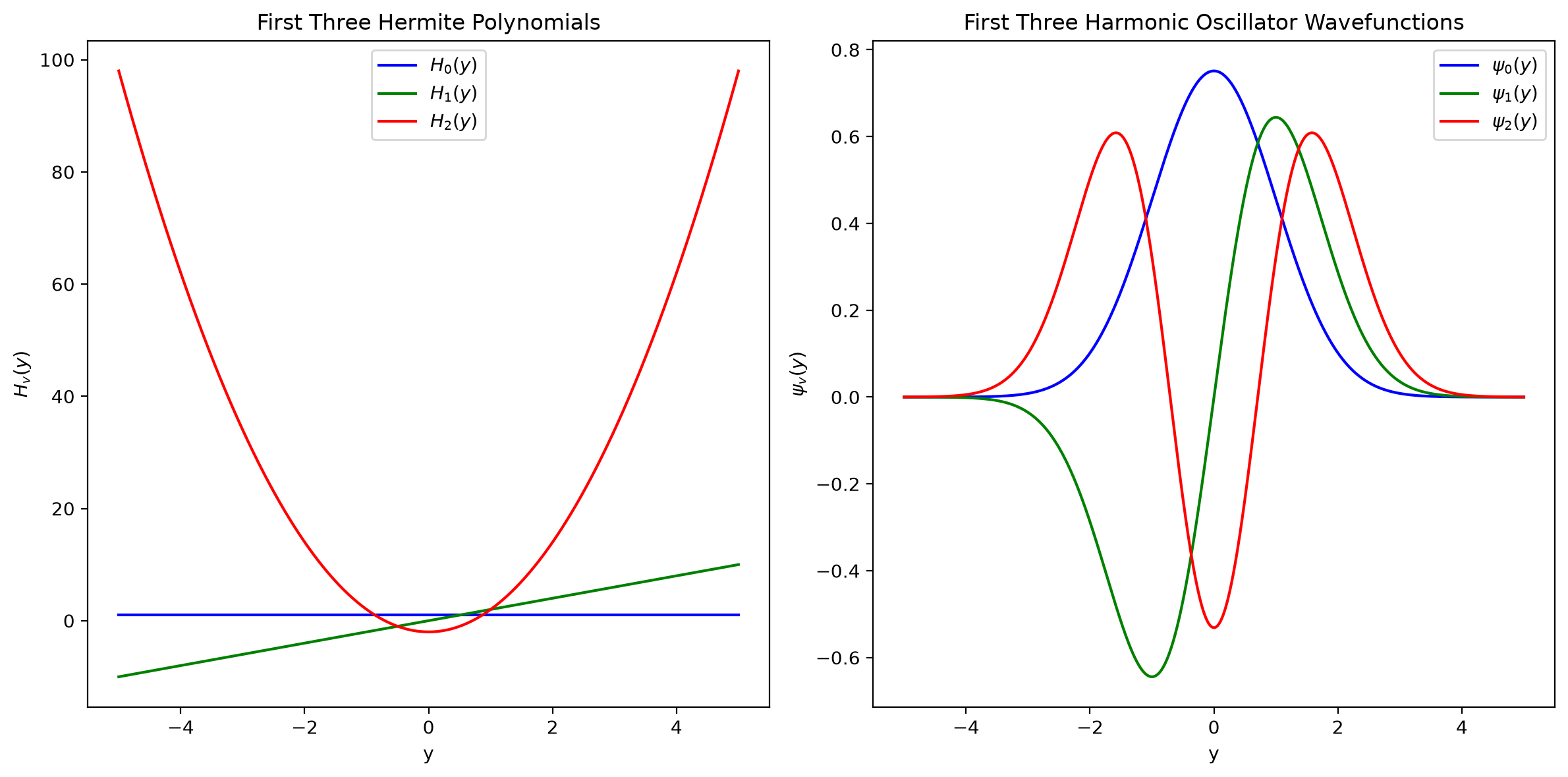
Source
import numpy as np
import matplotlib.pyplot as plt
from scipy.special import factorial

# Set constants
VMAX = 6
QPAD_FRAC = 1.3
SCALING = 0.7
COLOUR1 = 'blue'
COLOUR2 = 'red'

# Normalization constant and energy for vibrational state v
def N(v):
    return 1. / np.sqrt(np.sqrt(np.pi) * 2**v * factorial(v))

def get_E(v):
    return v + 0.5

# Generate Hermite polynomials
def make_Hr():
    Hr = [np.poly1d([1.]), np.poly1d([2., 0.])]
    for v in range(2, VMAX + 1):
        Hr.append(2 * np.poly1d([1., 0.]) * Hr[v-1] - 2 * (v-1) * Hr[v-2])
    return Hr

Hr = make_Hr()

# Get wavefunction and turning points
def get_psi(v, q):
    return N(v) * Hr[v](q) * np.exp(-q**2 / 2)

def get_turning_points(v):
    qmax = np.sqrt(2 * get_E(v))
    return -qmax, qmax

# Get potential energy
def get_potential(q):
    return q**2 / 2

# Plot function
def plot_func(ax, f, q, scaling=1, yoffset=0):
    ax.plot(q, f * scaling + yoffset, color=COLOUR1)
    ax.fill_between(q, f * scaling + yoffset, yoffset, f > 0, color=COLOUR1, alpha=0.5)
    ax.fill_between(q, f * scaling + yoffset, yoffset, f < 0, color=COLOUR2, alpha=0.5)

# Create subplots
fig, axs = plt.subplots(1, 2, figsize=(14, 8))

# Generate q range and potential
qmin, qmax = get_turning_points(VMAX)
xmin, xmax = QPAD_FRAC * qmin, QPAD_FRAC * qmax
q = np.linspace(qmin, qmax, 500)
V = get_potential(q)

# Plot potential and wavefunctions for both psi and |psi|^2
for ax, prob_plot in zip(axs, [False, True]):
    ax.plot(q, V, color='k', linewidth=1.5, label='Potential $V(q)$')
    for v in range(VMAX + 1):
        psi_v = get_psi(v, q)
        E_v = get_E(v)
        plot_func(ax, psi_v**2 if prob_plot else psi_v, q, scaling=SCALING * (1.5 if prob_plot else 1), yoffset=E_v)
        ax.text(s=f'$E_{v} = {E_v:.1f}$', x=qmax + 0.2, y=E_v + 0.1, va='center', ha='left')
        ax.axhline(y=E_v, color='gray', linestyle='--', alpha=0.7)  # Draw energy levels as dashed lines
    ax.set_xlim(xmin, xmax)
    ax.set_ylim(0, E_v + 0.5)
    ax.set_yticks([])
    ax.spines['top'].set_visible(False)
    ax.spines['right'].set_visible(False)
    ax.spines['left'].set_position('center')
    ax.set_xlabel('$q$', fontsize=12)
    ylabel = r'$|\psi(q)|^2$' if prob_plot else r'$\psi(q)$'
    ax.set_title(ylabel, fontsize=14)
    ax.legend()

plt.tight_layout()
plt.show()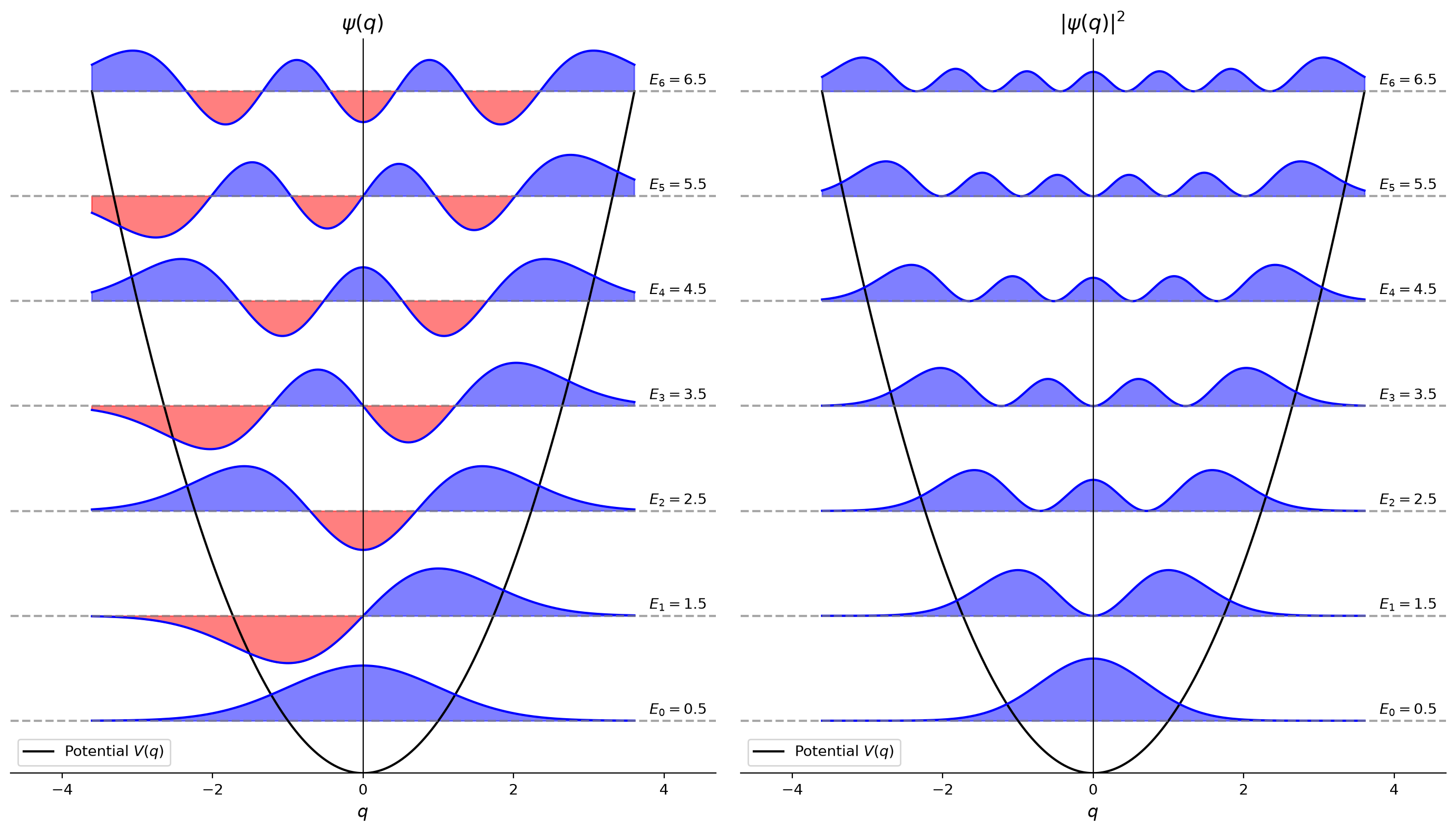
Odd/even symmetry of wavefunctions
Solutions with are even: .
Solutions with are odd: .
Consequences for evaluating integrals
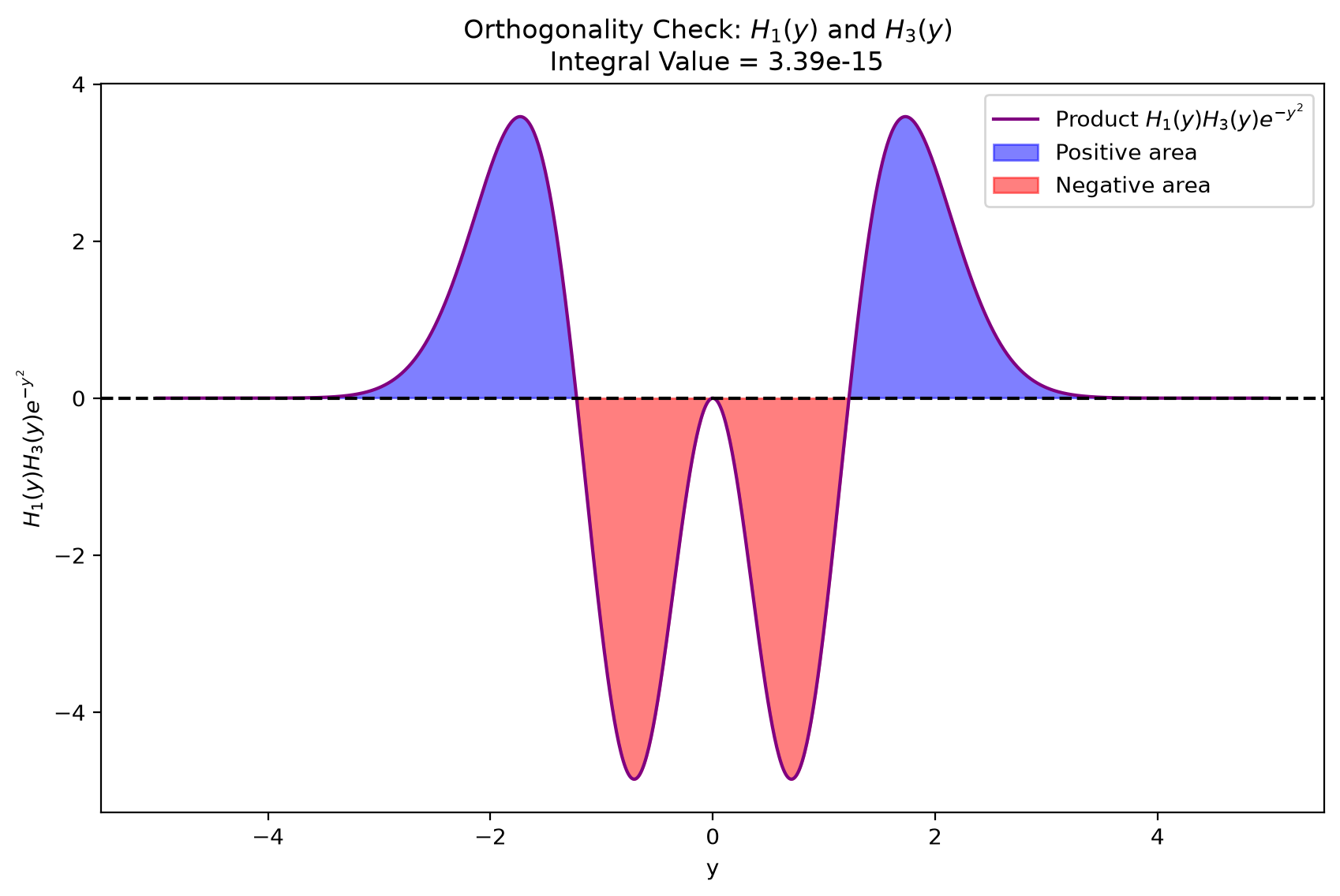
The integral of an odd function from to ( may be ) is zero.
This holds for all values
When you take the derivative of an odd (even) function you make it even (odd). For example, taking the derivative of the odd function gives , an even function.
As a result, we can set the following integral to zero:
And just like for , if we have two derivatives the expectation expression always returns an even function:
Visual illustration of orthogonality of eigenfunctions for quantum harmonic oscillator
Source
import numpy as np
import matplotlib.pyplot as plt
from scipy.special import hermite
from scipy.integrate import quad

# Hermite polynomial H_v(y) function
def H_v(v, y):
    return hermite(v)(y)

# Function to compute the product of H_v and H_v' for orthogonality check
def integrand(y, v1, v2):
    return H_v(v1, y) * H_v(v2, y) * np.exp(-y**2)

# Compute orthogonality integral
def check_orthogonality(v1, v2):
    # Integral of the product of two Hermite polynomials with exp(-y^2)
    integral, _ = quad(lambda y: integrand(y, v1, v2), -10, 10)  # Using finite limits for stability
    return integral

# Define the y range for plotting
y_values = np.linspace(-5, 5, 1000)

# Plot and check orthogonality for different pairs
def plot_orthogonality(v1, v2):
    H1 = H_v(v1, y_values)
    H2 = H_v(v2, y_values)
    product = H1 * H2 * np.exp(-y_values**2)

    fig, ax = plt.subplots(figsize=(10, 6))
    ax.plot(y_values, product, label=f'Product $H_{{{v1}}}(y) H_{{{v2}}}(y) e^{{-y^2}}$', color='purple')
    ax.fill_between(y_values, 0, product, where=(product > 0), color='blue', alpha=0.5, label='Positive area')
    ax.fill_between(y_values, 0, product, where=(product < 0), color='red', alpha=0.5, label='Negative area')

    # Orthogonality integral
    integral_value = check_orthogonality(v1, v2)
    ax.set_title(f'Orthogonality Check: $H_{{{v1}}}(y)$ and $H_{{{v2}}}(y)$ \n Integral Value = {integral_value:.2e}')
    ax.set_xlabel('y')
    ax.set_ylabel(f'$H_{{{v1}}}(y) H_{{{v2}}}(y) e^{{-y^2}}$')
    ax.axhline(0, color='black', linestyle='--')
    ax.legend()
    plt.show()

# Plot orthogonality for different cases
plot_orthogonality(1, 2)  # Odd vs Even: H_1(y) and H_2(y)
plot_orthogonality(0, 2)  # Even vs Even: H_0(y) and H_2(y)
plot_orthogonality(1, 3)  # Odd vs Odd: H_1(y) and H_3(y)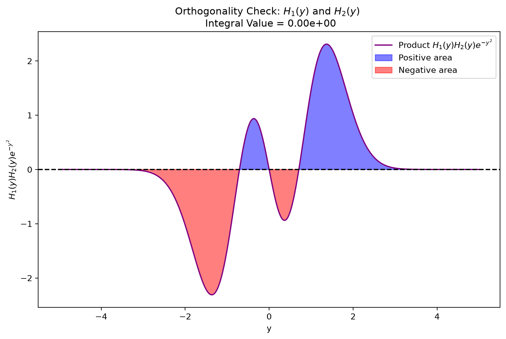
Tunneling and quantum-to-classical behavior
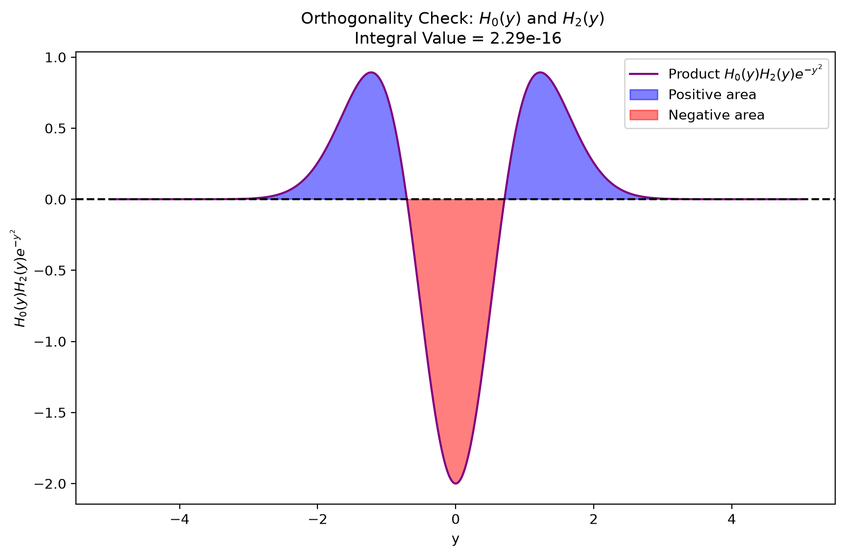
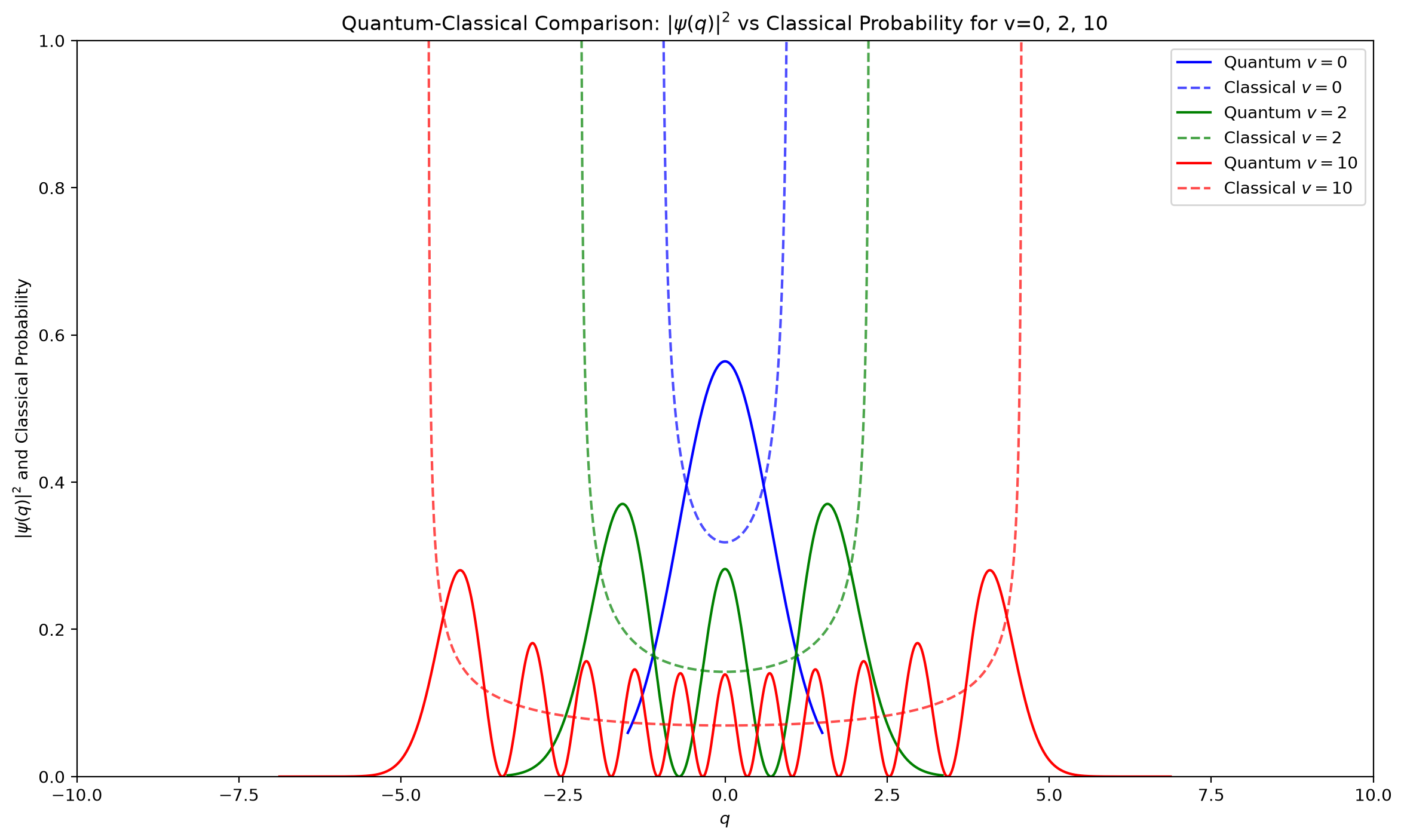
The tails of the wavefunctions penetrate into the potential barrier deeper than classical physics would allow. This phenomenon is called tunneling.
As we excite the system to higher levels, the probability distribution accumulates near the edges, thereby approaching the classical prediction.
Source
import numpy as np
import matplotlib.pyplot as plt
from scipy.special import factorial

# Set constants
QPAD_FRAC = 1.3
SCALING = 1.0
COLORS = ['blue', 'green', 'red']  # Different colors for each wavefunction
V_VALUES = [0, 2, 10]  # Vibrational quantum numbers to plot

# Normalization constant for vibrational state v
def normalization_constant(v):
    return 1. / np.sqrt(np.sqrt(np.pi) * 2**v * factorial(v))

# Energy for vibrational state v
def energy_level(v):
    return v + 0.5

# Generate Hermite polynomials
def make_Hermite_polynomials(v_max):
    Hr = [np.poly1d([1.]), np.poly1d([2., 0.])]
    for v in range(2, v_max + 1):
        Hr.append(2 * np.poly1d([1., 0.]) * Hr[v-1] - 2 * (v-1) * Hr[v-2])
    return Hr

# Get wavefunction for level v on grid q
def get_wavefunction(v, q, Hr):
    return normalization_constant(v) * Hr[v](q) * np.exp(-q**2 / 2)

# Get classical turning points for state v
def get_turning_points(v):
    qmax = np.sqrt(2 * energy_level(v))
    return -qmax, qmax

# Classical probability distribution for a harmonic oscillator
def classical_probability(v, q):
    qmax = np.sqrt(2 * energy_level(v))
    return 1 / (np.pi * np.sqrt(qmax**2 - q**2))

# Create plot
def plot_wavefunctions_square(v_values, colors):
    fig, ax = plt.subplots(figsize=(14, 8))

    # Generate Hermite polynomials up to the maximum v in v_values
    v_max = max(v_values)
    Hr = make_Hermite_polynomials(v_max)

    # Plot quantum probability distributions for each v
    for v, color in zip(v_values, colors):
        qmin, qmax = get_turning_points(v)
        q = np.linspace(qmin * 1.5, qmax * 1.5, 5000)  # Increased resolution
        psi_v_square = get_wavefunction(v, q, Hr)**2

        # Plot |psi|^2 for quantum mechanical probability
        ax.plot(q, psi_v_square, label=f'Quantum $v={v}$', color=color)

        # Plot classical probability for the same v
        q_classical = np.linspace(-qmax, qmax, 1000)
        classical_prob = classical_probability(v, q_classical)
        ax.plot(q_classical, classical_prob, '--', label=f'Classical $v={v}$', color=color, alpha=0.7)

    ax.set_xlim(-10, 10)
    ax.set_ylim([0, 1])
    ax.set_xlabel('$q$')
    ax.set_ylabel(r'$|\psi(q)|^2$ and Classical Probability')
    ax.set_title(r'Quantum-Classical Comparison: $|\psi(q)|^2$ vs Classical Probability for v=0, 2, 10')
    ax.legend()

    plt.show()

# Plot wavefunction squares for v=0, 10, 100, and classical probability
plot_wavefunctions_square(V_VALUES, COLORS)
/tmp/ipykernel_3161/317995826.py:38: RuntimeWarning: divide by zero encountered in divide
return 1 / (np.pi * np.sqrt(qmax**2 - q**2))
Problems
Solution
First we calculate ( is an even function, is odd, the integrand is odd overall):
For we have (by integration by parts or from a table of integrals):
For we have again by symmetry:
Note that the derivative of an even function is an odd function. For we have:
Finally, we can calculate :
Recall that the uncertainty principle states that .
Thus we can conclude that fulfills the Heisenberg uncertainty principle.
Solution
The harmonic vibration frequency is given in wavenumber units (). This must be converted according to . The previous example gives the expression for :
In considering spectroscopic data, it is convenient to express this in terms of :
In part (b) we apply the above expression to find the standard deviation of the carbon monoxide bond length in its ground vibrational state. First we need the reduced mass:
The standard deviation is now: