Energies of molecules
Molecules consisting of N nuclei and n electrons are described by wave functions that depend on 3(n+N) variables in 3D space. These coordinates, or degrees of freedom (DOF), are usefully broken down into different kinds of motion classified as translational, rotational, vibrational and electronic. Because molecules are microscopic objects, we expect all of these energies to be quantized. The relative spacings, however, differ significantly because of the boundary conditions that restrict the motions of these DOFs. This is why different kinds of spectroscopy exist for probing the specific degrees of freedom in molecules.
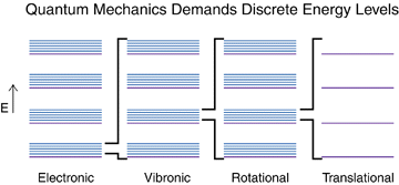
Figure 1:Energy levels associated with the different degrees of freedom in molecules.
3N Nuclear degrees of freedom
The Born-Oppenheimer approximation allows us to separate the nuclear and electronic degrees of freedom. The nuclear Hamiltonian for nuclei can now be written in such a way that the electronic part appears as a potential term:
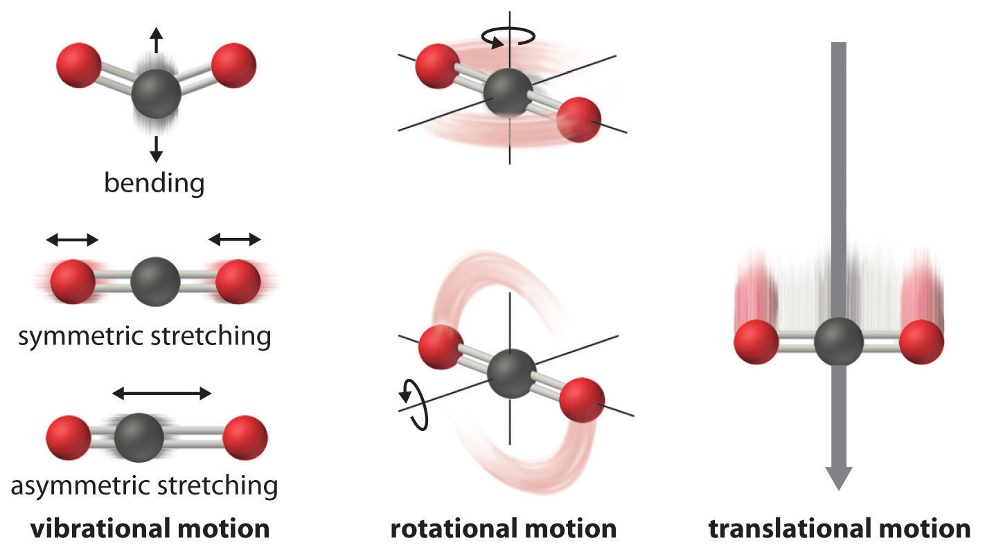
Figure 2:The different degrees of freedom in molecules: translational, rotational and vibrational motion.
In the absence of external electric or magnetic fields, the potential term depends only on the relative positions of the nuclei, as shown above, and not on the overall position of the molecule or its orientation in space. The above Hamiltonian can often be approximately written as a sum of the following terms:
where is the translational, the rotational, and the vibrational Hamiltonian. The translational and rotational terms have no potential part, but the vibrational part contains the potential , which depends on the distances between the nuclei.
In some cases the different degrees of freedom become coupled and one cannot use the following separation technique. Separation of means that we can write the wavefunction as a product:
Separation of degrees of freedom
The resulting three Schrödinger equations are then:
The translational part is not interesting, since there is no external potential or boundary condition that could lead to quantization (i.e., it produces a continuous spectrum).
On the other hand, the rotational part is subject to a cyclic boundary condition and the vibrational part to the potential , so we expect these to produce quantization, which can be probed by spectroscopic methods.
The original number of variables in the Hamiltonian is (i.e. the coordinates for each nucleus). We can neglect the translational motion, and we are left with coordinates.
To account for molecular rotation, three variables are required, or only two variables for a linear molecule. Therefore the vibrational part must have either variables for a non-linear molecule or variables for a linear molecule. These are referred to as vibrational degrees of freedom or internal coordinates.
Classical vibrations: the harmonic oscillator
Translations and rotations carry no potential energy, and the electronic problem is deferred to later chapters. The vibrational Hamiltonian is where the potential lives, and near any stable geometry that potential looks like a spring. Before quantizing the oscillator in the next lecture, we need full command of its classical mechanics.
Bead, spring and a wall
The classical harmonic oscillator is a system of a bead attached to a wall with a spring.
When the bead is displaced from its equilibrium or resting position to some point , it experiences a restoring force proportional to the displacement :
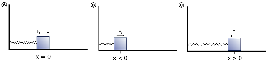
Figure 3:Harmonic motion governed by Hooke’s law. Any deviation from the equilibrium position is met with a restoring force, and in the absence of friction the bead oscillates indefinitely about equilibrium.
This is Hooke’s law, where the minus sign indicates that the direction of the force is always toward restoring the equilibrium location.
The constant characterizes the stiffness of the spring and is called the spring constant.
Solving harmonic oscillator problem
The classical equation of motion for a one-dimensional simple harmonic oscillator with a particle of mass m attached to a spring having spring constant k generates mechanical waves.
The introduced constant will be seen as the frequency of oscillations. Note that the frequency is inversely proportional to mass (heavier objects with the same spring constant oscillate more slowly around equilibrium) and increases with the spring constant (stiffer springs increase oscillations around equilibrium for the same mass).
The differential equation is a simple second-order, linear ODE which can be solved by the standard trick of plugging in an exponential and converting the problem to an algebraic equation. The solution is
The two constants are: , the amplitude of oscillations, and , a constant specifying the initial position of the bead.
Source
import numpy as np
import matplotlib.pyplot as plt
from matplotlib.animation import FuncAnimation
from IPython.display import HTML

def sho_anim(m, k=1.0, A=0.9, phi=0.0, duration=4.0, fps=30):
    ω = np.sqrt(k/m)
    t = np.linspace(0, duration, int(fps*duration))
    x = A*np.sin(ω*t + phi)

    fig, axes = plt.subplots(1, 2, figsize=(8, 2.5))
    ax_mass, ax_wave = axes

    # --- left: oscillating mass ---
    ax_mass.set_xlim(-1.2, 1.2)
    ax_mass.set_ylim(-0.5, 0.5)
    ax_mass.axis("off")
    ax_mass.set_title(f"Mass–Spring (m={m:g})")
    (mass_point,) = ax_mass.plot([], [], "o", ms=12)
    (trace_line,) = ax_mass.plot([], [], lw=2)

    # --- right: sinusoidal wave ---
    ax_wave.set_xlim(0, duration)
    ax_wave.set_ylim(-1.2*A, 1.2*A)
    ax_wave.set_xlabel("time t")
    ax_wave.set_ylabel("x(t)")
    ax_wave.grid(True, ls="--", alpha=0.4)
    ax_wave.set_title("x(t) = A sin (ωt + φ)")
    (wave_line,) = ax_wave.plot([], [], lw=2)
    (wave_point,) = ax_wave.plot([], [], "o")

    def init():
        for line in (mass_point, trace_line, wave_line, wave_point):
            line.set_data([], [])
        return mass_point, trace_line, wave_line, wave_point

    def update(i):
        xi = x[i]
        mass_point.set_data([xi], [0])
        trace_line.set_data(x[:i+1], np.zeros(i+1))
        wave_line.set_data(t[:i+1], x[:i+1])
        wave_point.set_data([t[i]], [xi])
        return mass_point, trace_line, wave_line, wave_point

    return FuncAnimation(fig, update, init_func=init, frames=len(t), interval=1000/fps, blit=True)

# --- Two animations: normal mass and heavier mass ---
anim1 = sho_anim(m=1.0, duration=10.0)
anim2 = sho_anim(m=10.0, duration=10.0)  # slower oscillation

# Inline display in Jupyter / Jupyter Book
plt.close()  # Prevents static display of the last frame
HTML(anim1.to_jshtml() + "<br><hr><br>" + anim2.to_jshtml())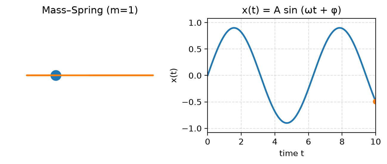
Energy of the harmonic oscillator
In classical mechanics, when we have a conservative system (no friction, energy conserved) the force is the gradient of a potential energy
This means the steeper the potential, the larger the force, and the minus sign indicates that the force restores the system to its equilibrium position.
The potential energy can be obtained by integrating:
Thus the potential energy for a simple harmonic oscillator is a parabolic function of displacement. It is convenient to set and measure potential energy relative to the equilibrium state .
The total energy, consisting of kinetic and potential energies, will be used to obtain the Schrodinger equation.
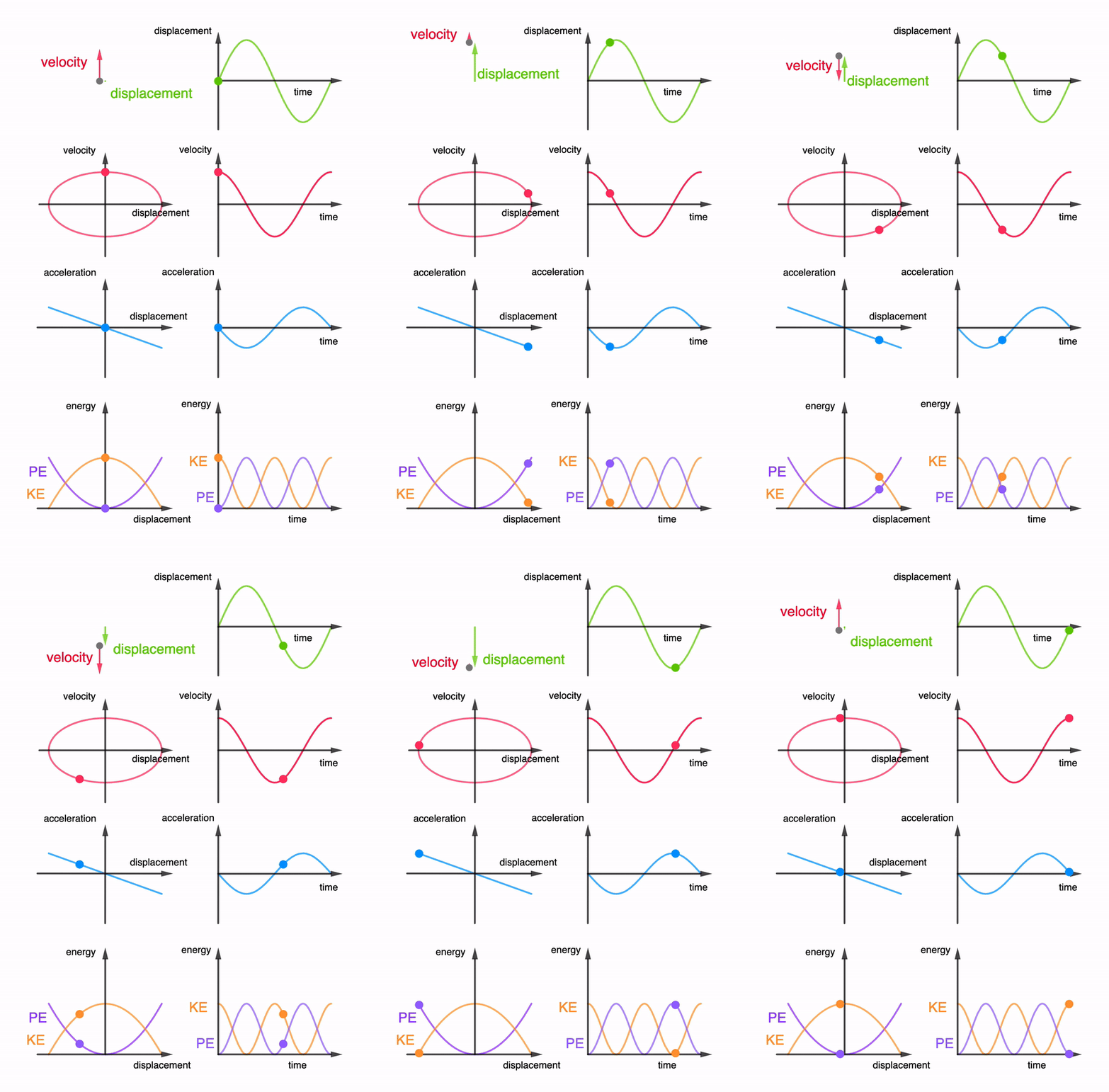
Figure 4:A harmonic oscillator in vacuum is conservative: kinetic and potential energy interconvert with no total energy dissipated into the environment. Position , velocity , and acceleration all oscillate at the same constant frequency but with different amplitudes.
Diatomic molecules and two-body problem
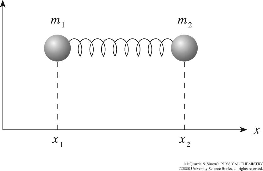
Figure 5:We can reduce the two-body problem of vibrating atoms to a one-body problem of a single particle with an effective reduced mass , so .
Derivation
Equations of motion for diatomic molecule modeled as beads bound by a spring are:
where , a reflection of Newton’s third law. By introducing more convenient coordinates in the form of the relative distance and the center of mass , we now reduce the two-body problem to a one-body problem.
The diatomic molecule is stable because the same force acts on both ends
By expressing the equations of motion in terms of the center of mass, we find that the center of mass moves freely without acceleration.
Next, by taking the difference between the coordinates and , we express the equations of motion in terms of the relative distance
This equation looks identical to the problem of a bead anchored to a wall with a spring. We have thus managed to reduce the two-body problem to a one-body problem by replacing the masses of the bodies with a reduced mass , so
### Beads and springs model of molecules

- Before discussing the harmonic oscillator approximation, let us reflect on when it is a good approximation and under which circumstances it breaks down. For an arbitrary potential energy function of $x$, we can carry out a Taylor expansion around the equilibrium bond length $x_0$, obtaining an infinite series.

$$U(x) = U(x_0)+U'(x_0)(x-x_0)+\frac{1}{2!}U''(x_0)(x-x_0)^2+\frac{1}{3!}U'''(x_0)(x-x_0)^3+...$$


:::{figure} images/harm_approx.png
:label: fig-classical-harmonic-oscillator-4
:alt: harmls
:width: 300px

Deviation of the true potential (blue) from the simple harmonic approximation (red), with the cubic correction shown in green.
Setting the energy scale relative to and recognizing that the first derivative vanishes at the minimum , we have
Hence we see that the harmonic approximation keeps only the first non-vanishing term! Furthermore, the spring constant and the subsequent anharmonicity constants such as are higher-order derivatives of the potential energy. That is, the more nonlinear the potential, the larger the contribution of these terms. Conversely, the closer the potential is to a quadratic form, the more accurate the harmonic assumption.
Source
import numpy as np
import matplotlib.pyplot as plt

# Define the range for x values, focusing on the dissociation region
x = np.linspace(0, 2.5, 500)

# Define the harmonic potential (quadratic term)
harmonic = 0.5 * x**2

# Define the harmonic + cubic potential
harmonic_cubic = 0.5 * x**2 - 0.2 * x**3

# Define the harmonic + cubic + quartic potential
harmonic_cubic_quartic = 0.5 * x**2 - 0.2 * x**3 + 0.05 * x**4

# Define the harmonic + cubic + quartic + higher-order polynomial (5th and 6th order)
polynomial_approx = 0.5 * x**2 - 0.2 * x**3 + 0.05 * x**4 - 0.01 * x**5 + 0.001 * x**6

# Define the Morse potential
def morse_potential(x, D=1, a=1):
    return D * (1 - np.exp(-a * x))**2

# Set parameters for Morse potential
D = 1  # Depth of the potential well
a = 1  # Width of the potential well

# Compute Morse potential
morse = morse_potential(x, D, a)

# Plot all the potentials, showing progression
plt.figure(figsize=(8, 6))

# Harmonic only
plt.plot(x, harmonic, label='Harmonic: $0.5  x^2$', color='b', lw=2)

# Harmonic + Cubic
plt.plot(x, harmonic_cubic, label='Harmonic + Cubic: $0.5  x^2 - 0.2  x^3$', color='g', lw=2)

# Harmonic + Cubic + Quartic
plt.plot(x, harmonic_cubic_quartic, label='Harmonic + Cubic + Quartic: $0.5  x^2 - 0.2  x^3 + 0.05  x^4$', color='r', lw=2)

# Polynomial approximation (up to 6th order)
plt.plot(x, polynomial_approx, label='Polynomial Approx (up to $x^6$)', color='c', lw=2)

# Morse potential
plt.plot(x, morse, label='Morse Potential', color='k', lw=3)

# Add labels and legend
plt.title('Polynomial Approximation of Harmonic Oscillator vs. Morse Potential')
plt.xlabel('x (dissociation region)')
plt.ylabel('Potential Energy')
plt.axhline(0, color='black',linewidth=0.5)
plt.axvline(0, color='black',linewidth=0.5)
plt.grid(True)
plt.legend()
plt.ylim([0, 2])
(0.0, 2.0)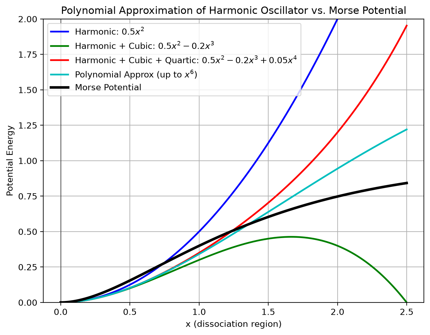
Problems
Problem 1: Count the degrees of freedom
How many vibrational modes do (a) HCl, (b) ammonia NH (nonlinear), and (c) acetylene CH (linear) have?
Solution
(a) HCl: , linear, so vibration (the bond stretch). (b) NH: , nonlinear, so vibrations. (c) CH: , linear, so vibrations.
Problem 2: Vibrational frequency of HCl
The force constant of the HCl bond is N/m. Compute the reduced mass and the angular frequency , and convert to a wavenumber .
Solution
, matching the observed HCl stretch near 2886 cm.
Problem 3: Isotope shift
Without recomputing from scratch, predict how changes when HCl is replaced by DCl. The force constant does not change. Why not?
Problem 4: Spring constant from a potential
A bond is described by (the Morse potential, with the displacement from equilibrium). Taylor expand around to show that the effective spring constant is .
Problem 5: Energy bookkeeping
A classical oscillator has amplitude . At what displacement is the energy split exactly half kinetic, half potential? Sketch , , and on one plot.