
This demo uses the following libraries (already installed for the site build; on your own machine,
pip install pyscf py3Dmol plotly)
from pyscf import gto   # Used to define a molecule
from pyscf import scf   # Used to perform HF calculations
from pyscf import mp    # Used to perform Møller–Plesset PT calculations
from pyscf import cc    # Used to perfrom Coupled Cluster calculations
from pyscf import mcscf # Used to perform multireference calculations
Overview of Basis sets used in calculations
Minimal & small
sto-3g– very small, qualitative (what you already used).sto-6g– still minimal, but better approximation to Slater orbitals; improved E(R) shape.
Split-valence Pople sets
3-21g– first split-valence; cheap, decent improvement over STOs.6-31g– classic workhorse; much better bond length and well depth for H₂.
With polarization
6-31g*or6-31g(d)– adds d-functions on heavy atoms (not needed for H₂).6-31g**or6-31g(d,p)– adds p-functions on H; recommended for H₂ to improve curvature and accuracy.
Correlation-consistent (Dunning) sets
cc-pVDZ– correlation-consistent double-ζ; very good HF curve.cc-pVTZ– triple-ζ; near basis-set limit for HF on H₂.aug-cc-pVDZ– includes diffuse functions; useful for exploring dissociation tail / anionic behavior.
Diatomics
import numpy as np
import matplotlib.pyplot as plt
from pyscf import gto, scf, tools

def compute_h2_bond_curve(distances, basis='sto-3g'):
    """
    Computes the total energy of H2 molecule at various bond distances.

    Parameters:
    - distances (array-like): List of H-H bond distances to calculate energy.
    - basis (str): Basis set for the calculation.

    Returns:
    - energies (list): Total electronic energies for each bond distance.
    - mo_energies_list (list of lists): Molecular orbital energies for each distance.
    - mo_coeffs_list (list of arrays): Molecular orbital coefficients for each distance.
    """
    energies = []
    mo_energies_list = []
    mo_coeffs_list = []

    for r in distances:
        mol = gto.Mole()
        mol.atom = f'H 0 0 0; H 0 0 {r}'
        mol.basis = basis
        mol.spin = 0  # Singlet state
        mol.build()

        # Perform Hartree-Fock calculation
        mf = scf.RHF(mol)
        total_energy = mf.kernel()

        # Store results
        energies.append(total_energy)
        mo_energies_list.append(mf.mo_energy)
        mo_coeffs_list.append(mf.mo_coeff)

        print(f"Bond distance: {r:.2f} Å, Total Energy: {total_energy:.6f} Hartree")

    return energies, mo_energies_list, mo_coeffs_list

def plot_bond_curve(distances, energies):
    """
    Plots the bond energy curve of H2 molecule.

    Parameters:
    - distances (array-like): H-H bond distances.
    - energies (list): Total electronic energies for each bond distance.
    """
    plt.figure(figsize=(8, 5))
    plt.plot(distances, energies, marker='o', label='Total Energy (HF)')
    plt.xlabel('H-H Bond Distance (Å)')
    plt.ylabel('Total Energy (Hartree)')
    plt.title('Bond Curve for H2 (HF/STO-3G)')
    plt.grid(True)
    plt.legend()
    plt.show()

def plot_molecular_orbitals(distances, mo_energies_list):
    """
    Plots the molecular orbital energies as a function of bond distance.

    Parameters:
    - distances (array-like): H-H bond distances.
    - mo_energies_list (list of lists): Molecular orbital energies for each distance.
    """
    plt.figure(figsize=(8, 5))
    for i in range(len(mo_energies_list[0])):  # Number of orbitals
        orbital_energies = [mo_energies[i] for mo_energies in mo_energies_list]
        plt.plot(distances, orbital_energies, marker='o', label=f'MO {i+1}')

    plt.xlabel('H-H Bond Distance (Å)')
    plt.ylabel('Molecular Orbital Energy (Hartree)')
    plt.title('Molecular Orbital Energies for H2 (HF/STO-3G)')
    plt.grid(True)
    plt.legend()
    plt.show()
# Define bond distances (in Ångstroms)
distances = np.linspace(0.5, 3.0, 20) # From 0.5 to 3.0 Å
# Run the bond curve calculation
energies, mo_energies_list, mo_coeffs_list = compute_h2_bond_curve(distances)
# Plot the bond curve
plot_bond_curve(distances, energies)
# Plot the molecular orbital energies as a function of bond distance
plot_molecular_orbitals(distances, mo_energies_list)converged SCF energy = -1.04299627454009
Bond distance: 0.50 Å, Total Energy: -1.042996 Hartree
converged SCF energy = -1.10962287714076
Bond distance: 0.63 Å, Total Energy: -1.109623 Hartree
converged SCF energy = -1.1151049457252
Bond distance: 0.76 Å, Total Energy: -1.115105 Hartree
converged SCF energy = -1.09311721487025
Bond distance: 0.89 Å, Total Energy: -1.093117 Hartree
converged SCF energy = -1.05859984694162
Bond distance: 1.03 Å, Total Energy: -1.058600 Hartree
converged SCF energy = -1.0184750668009
Bond distance: 1.16 Å, Total Energy: -1.018475 Hartree
converged SCF energy = -0.976475042485522
Bond distance: 1.29 Å, Total Energy: -0.976475 Hartree
converged SCF energy = -0.934934347558081
Bond distance: 1.42 Å, Total Energy: -0.934934 Hartree
converged SCF energy = -0.895332352040937
Bond distance: 1.55 Å, Total Energy: -0.895332 Hartree
converged SCF energy = -0.858539335922428
Bond distance: 1.68 Å, Total Energy: -0.858539 Hartree
converged SCF energy = -0.825003227962735
Bond distance: 1.82 Å, Total Energy: -0.825003 Hartree
converged SCF energy = -0.794885434688666
Bond distance: 1.95 Å, Total Energy: -0.794885 Hartree
converged SCF energy = -0.768150987030312
Bond distance: 2.08 Å, Total Energy: -0.768151 Hartree
converged SCF energy = -0.744632766213529
Bond distance: 2.21 Å, Total Energy: -0.744633 Hartree
converged SCF energy = -0.724083718963794
Bond distance: 2.34 Å, Total Energy: -0.724084 Hartree
converged SCF energy = -0.706219811199347
Bond distance: 2.47 Å, Total Energy: -0.706220 Hartree
converged SCF energy = -0.690751272496288
Bond distance: 2.61 Å, Total Energy: -0.690751 Hartree
converged SCF energy = -0.67740092568721
Bond distance: 2.74 Å, Total Energy: -0.677401 Hartree
converged SCF energy = -0.665911797817778
Bond distance: 2.87 Å, Total Energy: -0.665912 Hartree
converged SCF energy = -0.656048251145591
Bond distance: 3.00 Å, Total Energy: -0.656048 Hartree
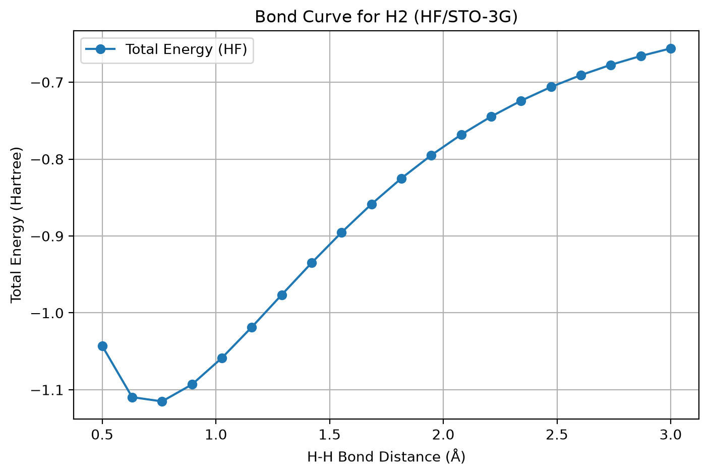
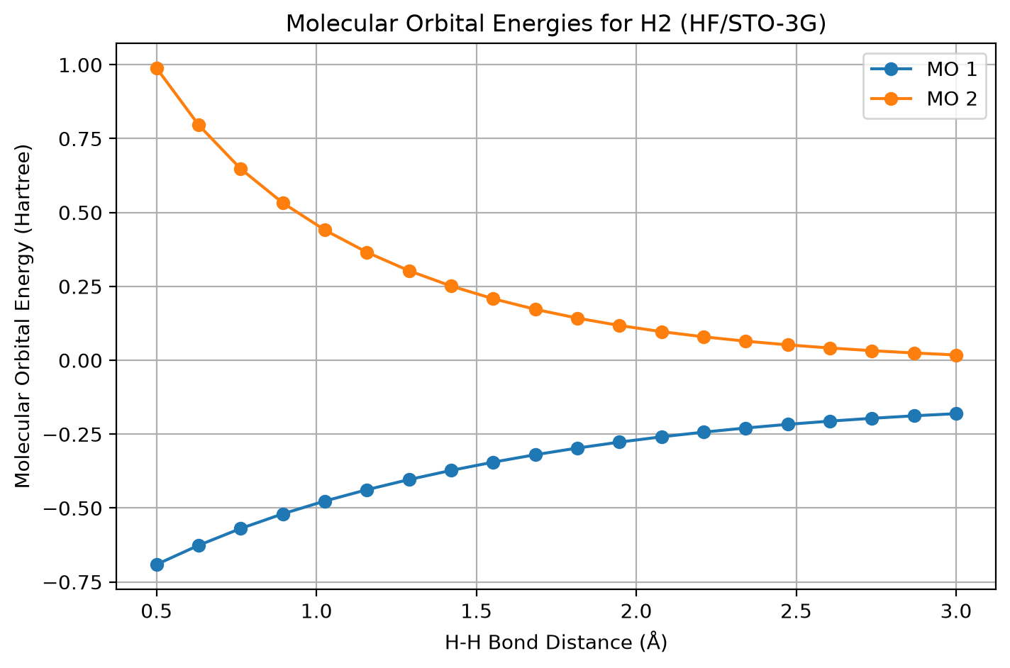
import numpy as np
from pyscf import gto, scf, tools
import py3Dmol  # For 3D visualization of orbitals

def visualize_h2_mo_cubes(bond_distance=0.74, basis='sto-3g', mo_index=0, output_cube_file='mo.cube'):
    """
    Generate and visualize cube files for molecular orbitals of H2.

    Parameters:
    - bond_distance (float): H-H bond distance (in Ångstroms).
    - basis (str): Basis set for the calculation (e.g., 'sto-3g', '6-31g').
    - mo_index (int): Index of the molecular orbital to visualize (0-indexed).
    - output_cube_file (str): The name of the cube file to save.
    """
    # 1. Build the H2 molecule
    mol = gto.Mole()
    mol.atom = f'H 0 0 0; H 0 0 {bond_distance}'
    mol.basis = basis
    mol.spin = 0  # Singlet state
    mol.build()

    # 2. Perform Hartree-Fock calculation
    mf = scf.RHF(mol)
    mf.kernel()

    # 3. Generate cube file for the specified molecular orbital (MO)
    print(f"Generating cube file for MO {mo_index + 1} (0-indexed as {mo_index})")
    tools.cubegen.orbital(mol, output_cube_file, mf.mo_coeff[:, mo_index], nx=80, ny=80, nz=80)

    # 4. Visualize the molecular orbital using py3Dmol
    print(f"Visualizing cube file: {output_cube_file}")
    cube_view = py3Dmol.view(width=400, height=400)
    with open(output_cube_file, 'r') as cube_file:
        cube_data = cube_file.read()

    # Add isosurfaces for positive and negative parts of the orbital
    cube_view.addVolumetricData(cube_data, "cube", {'isoval': -0.03, 'color': "red", 'opacity': 0.85})
    cube_view.addVolumetricData(cube_data, "cube", {'isoval': 0.03, 'color': "blue", 'opacity': 0.85})

    # Add the molecular structure as well
    cube_view.addModel(mol.tostring(format="xyz"), 'xyz')
    cube_view.setStyle({'stick': {}, 'sphere': {'radius': 0.4}})
    cube_view.setBackgroundColor('0xeeeeee')
    cube_view.show()
# Set the bond distance, basis, and the index of the molecular orbital to visualize
visualize_h2_mo_cubes(bond_distance=0.74, basis='sto-3g', mo_index=1, output_cube_file='mo_1.cube') # MO 1converged SCF energy = -1.11675930739643
Generating cube file for MO 2 (0-indexed as 1)
Visualizing cube file: mo_1.cube
Build and Visualize Benzene
mol_xyz = """H      1.2194     -0.1652      2.1600
  C      0.6825     -0.0924      1.2087
  C     -0.7075     -0.0352      1.1973
  H     -1.2644     -0.0630      2.1393
  C     -1.3898      0.0572     -0.0114
  H     -2.4836      0.1021     -0.0204
  C     -0.6824      0.0925     -1.2088
  H     -1.2194      0.1652     -2.1599
  C      0.7075      0.0352     -1.1973
  H      1.2641      0.0628     -2.1395
  C      1.3899     -0.0572      0.0114
  H      2.4836     -0.1022      0.0205"""

mol = gto.M(atom=mol_xyz, basis="sto3g", verbose=3)
import py3Dmol
xyz_view = py3Dmol.view(width=400,height=400)
xyz_view.addModel(mol.tostring(format="xyz"),'xyz')
xyz_view.setStyle({'stick':{}, "sphere":{"radius":0.4}})
xyz_view.setBackgroundColor('0xeeeeee')
xyz_view.show()
#
# Use your mouse to interact with the molecule!
#Run calculations
# Run HF and save the results
mf = scf.RHF(mol).run()

# In Jupyter notebooks you can hover over methods to see docstrings or you can print the docstrings out!
#print(mf.__doc__)
converged SCF energy = -227.890481261003
Visualize Results
import plotly.express as px

# Plot the MO Occupations
fig = px.line(y=mf.mo_occ, markers=True, title="Molecular Orbital (MO) Occupations")
fig.update_layout(xaxis_title="Orbital Index (0-Based)", yaxis_title="MO Occupation")
fig.show()# Plot the MO Energies (i.e. eigenvalues of the Fock matrix)
fig = px.line(y=mf.mo_energy, markers=True, title="Molecular Orbital (MO) Energies")
fig.update_layout(xaxis_title="Orbital Index (0-Based)", yaxis_title="MO Energies")
fig.show()from pyscf.tools import cubegen
cubegen.orbital(mol, 'mo.cube', mf.mo_coeff[:,18]); # 42 electrons so 21 occupied orbitals
cube_view = py3Dmol.view(width=400,height=400)
cube_view.addVolumetricData(open("mo.cube").read(), "cube", {'isoval': -0.03, 'color': "red", 'opacity': 0.85})
cube_view.addVolumetricData(open("mo.cube").read(), "cube", {'isoval': 0.03, 'color': "blue", 'opacity': 0.85})
cube_view.addModel(mol.tostring(format="xyz"),'xyz')
cube_view.setStyle({'stick':{}, "sphere":{"radius":0.4}})
cube_view.setBackgroundColor('0xeeeeee')
cube_view.show()
#
# Use your mouse to interact with the molecule!
#| Region | Orbital indices | Type | Comment |
|---|---|---|---|
| Very low | 0–5 | C 1s core | Flat band, strongly bound |
| Middle | 6–20 | σ bonding | σ-framework in the ring |
| Gap | ~21 | Highest occupied π | Aromatic HOMO |
| High | 22–35 | π*/σ* | Virtual MOs |
Short Survey of more acurate methods
from pyscf import gto, scf, dft, mp, cc, fci
import py3Dmol
import plotly.express as px
# Experimental geometry of gas-phase water
# Ref: https://cccbdb.nist.gov/expgeom2x.asp
mol_xyz = """O 0.0000 0.0000 0.1173
H 0.0000 0.7572 -0.4692
H 0.0000 -0.7572 -0.4692"""
mol = gto.M(
atom=mol_xyz,
basis="6-31g",
verbose=4,
charge=0, # 0 by default
spin=0, # 0 by default, defined as (n_up - n_down)
symmetry=True, # False by default
)System: uname_result(system='Linux', node='runnervm76f27', release='6.17.0-1022-azure', version='#22-Ubuntu SMP Mon Jul 27 17:24:03 UTC 2026', machine='x86_64') Threads 4
Python 3.13.15 (main, Aug 6 2026, 02:15:18) [GCC 13.3.0]
numpy 2.5.2 scipy 1.18.0 h5py 3.16.0
Date: Thu Aug 20 20:31:26 2026
PySCF version 2.14.0
PySCF path /opt/hostedtoolcache/Python/3.13.15/x64/lib/python3.13/site-packages/pyscf
[CONFIG] conf_file None
[INPUT] verbose = 4
[INPUT] num. atoms = 3
[INPUT] num. electrons = 10
[INPUT] charge = 0
[INPUT] spin (= nelec alpha-beta = 2S) = 0
[INPUT] symmetry True subgroup None
[INPUT] Mole.unit = angstrom
[INPUT] Symbol X Y Z unit X Y Z unit Magmom
[INPUT] 1 O 0.000000000000 0.000000000000 0.117300000000 AA 0.000000000000 0.000000000000 0.221664874411 Bohr 0.0
[INPUT] 2 H 0.000000000000 0.757200000000 -0.469200000000 AA 0.000000000000 1.430900621521 -0.886659497646 Bohr 0.0
[INPUT] 3 H 0.000000000000 -0.757200000000 -0.469200000000 AA 0.000000000000 -1.430900621521 -0.886659497646 Bohr 0.0
nuclear repulsion = 9.1895337629349
point group symmetry = C2v
symmetry origin: [0. 0. 0.]
symmetry axis x: [-1. -0. -0.]
symmetry axis y: [0. 1. 0.]
symmetry axis z: [0. 0. 1.]
num. orbitals of irrep A1 = 7
num. orbitals of irrep B1 = 2
num. orbitals of irrep B2 = 4
number of shells = 9
number of NR pGTOs = 30
number of NR cGTOs = 13
basis = 6-31g
ecp = {}
CPU time: 19.14
xyz_view = py3Dmol.view(width=400,height=400)
xyz_view.addModel(mol.tostring(format="xyz"),'xyz')
xyz_view.setStyle({'stick':{}, "sphere":{"radius":0.4}})
xyz_view.setBackgroundColor('0xeeeeee')
xyz_view.show()Hartree-Fock
Hatree-Fock (HF) is the starting point of the most of quantum chemistry
We variationally optimize the orbitals for a single Slater determinint
Working in the basis of atom-centered basis function we solve the Roothaan-Hall equations
See the PySCF user guide and examples for more info.
mymf = scf.RHF(mol).run()
******** <class 'pyscf.scf.hf_symm.SymAdaptedRHF'> ********
method = SymAdaptedRHF
initial guess = minao
damping factor = 0
level_shift factor = 0
DIIS = <class 'pyscf.scf.diis.CDIIS'>
diis_start_cycle = 1
diis_space = 8
diis_damp = 0
SCF conv_tol = 1e-09
SCF conv_tol_grad = None
SCF max_cycles = 50
direct_scf = True
direct_scf_tol = 1e-13
chkfile to save SCF result = /tmp/tmp51ai18jp
max_memory 4000 MB (current use 395 MB)
Freeze 0 electrons in irreps []
10 free electrons in irreps A1 B1 B2
Set gradient conv threshold to 3.16228e-05
Initial guess from minao.
init E= -75.8343030732679
HOMO (B1) = -0.474622307499056 LUMO (A1) = 0.124028813320098 gap/eV = 16.29013
cycle= 1 E= -75.9458238773405 delta_E= -0.112 |g|= 0.419 |ddm|= 1.19
HOMO (B1) = -0.41446039447561 LUMO (A1) = 0.209091679575772 gap/eV = 16.96772
cycle= 2 E= -75.9747569680174 delta_E= -0.0289 |g|= 0.226 |ddm|= 0.406
HOMO (B1) = -0.503724607052101 LUMO (A1) = 0.197910489056946 gap/eV = 19.09246
cycle= 3 E= -75.9837994485706 delta_E= -0.00904 |g|= 0.022 |ddm|= 0.142
HOMO (B1) = -0.499873983490941 LUMO (A1) = 0.203806292491575 gap/eV = 19.14812
cycle= 4 E= -75.983968312152 delta_E= -0.000169 |g|= 0.00351 |ddm|= 0.0223
HOMO (B1) = -0.501170980205032 LUMO (A1) = 0.203672006137031 gap/eV = 19.17975
cycle= 5 E= -75.9839743119537 delta_E= -6e-06 |g|= 0.000534 |ddm|= 0.00506
HOMO (B1) = -0.501373592709125 LUMO (A1) = 0.203643081946627 gap/eV = 19.18448
cycle= 6 E= -75.983974470941 delta_E= -1.59e-07 |g|= 5.35e-05 |ddm|= 0.000938
HOMO (B1) = -0.501372091345514 LUMO (A1) = 0.203641391321118 gap/eV = 19.18439
cycle= 7 E= -75.9839744725996 delta_E= -1.66e-09 |g|= 1.24e-05 |ddm|= 9.81e-05
HOMO (B1) = -0.501368130501562 LUMO (A1) = 0.203641216029915 gap/eV = 19.18428
cycle= 8 E= -75.9839744727203 delta_E= -1.21e-10 |g|= 1.54e-06 |ddm|= 3.21e-05
HOMO (B1) = -0.501368365983406 LUMO (A1) = 0.203640958576327 gap/eV = 19.18428
Extra cycle E= -75.9839744727217 delta_E= -1.32e-12 |g|= 7.11e-07 |ddm|= 2.46e-06
converged SCF energy = -75.9839744727217
Density Functional Theory
In Density Functional Theory (DFT), the electron density of a reference noninteracting system is used to represent the density of the true interacting system.
The formulation resembles HF with a different effective Fock potential.
This effective potential depends on the density functional approximation which is chosen by the user.
PySCF gives users the access to a large number of functionals through the libxc and xcfun libraries.
See the PySCF user guide and examples for more info.
Møller–Plesset perturbation theory
Perturbative corrections to the Hartree-Fock approximation.
See the PySCF user guide and examples for more info.
mymp2 = mp.MP2(mymf).run()
******** <class 'pyscf.mp.mp2.RMP2'> ********
nocc = 5, nmo = 13
max_memory 4000 MB (current use 398 MB)
E(RMP2) = -76.1128253908809 E_corr = -0.128850918159199
E(SCS-RMP2) = -76.1124627493824 E_corr = -0.128488276660723
E_corr(same-spin) = -0.0301532597657486
E_corr(oppo-spin) = -0.0986976583934503
Coupled Cluster
Perturbative method that improves on the Hartree-Fock approximation.
Coupled Cluster Singles and Doubles (CCSD) includes single and double excitation on top of the HF wave function.
Accuracy can be improved by including triples perturbatively (CCSD(T)).
Non-variational, but size extensive description of ground states. For excited states, see EOM-CCSD.
See the PySCF user guide and examples for more info.
mycc = cc.CCSD(mymf).run()
******** <class 'pyscf.cc.ccsd.CCSD'> ********
CC2 = 0
CCSD nocc = 5, nmo = 13
max_cycle = 50
direct = 0
conv_tol = 1e-07
conv_tol_normt = 1e-05
diis_space = 6
diis_start_cycle = 0
diis_start_energy_diff = 1e+09
max_memory 4000 MB (current use 398 MB)
Init t2, MP2 energy = -76.1128253971341 E_corr(MP2) -0.128850924412438
Init E_corr(CCSD) = -0.128850924412628
cycle = 1 E_corr(CCSD) = -0.131108130968237 dE = -0.00225720656 norm(t1,t2) = 0.0228787
cycle = 2 E_corr(CCSD) = -0.133971459205635 dE = -0.00286332824 norm(t1,t2) = 0.00827705
cycle = 3 E_corr(CCSD) = -0.135274692633285 dE = -0.00130323343 norm(t1,t2) = 0.00329509
cycle = 4 E_corr(CCSD) = -0.135395198809583 dE = -0.000120506176 norm(t1,t2) = 0.000547317
cycle = 5 E_corr(CCSD) = -0.13538272686884 dE = 1.24719407e-05 norm(t1,t2) = 0.000202845
cycle = 6 E_corr(CCSD) = -0.135379406531295 dE = 3.32033755e-06 norm(t1,t2) = 5.06174e-05
cycle = 7 E_corr(CCSD) = -0.135379879258623 dE = -4.72727328e-07 norm(t1,t2) = 1.08852e-05
cycle = 8 E_corr(CCSD) = -0.135379510430962 dE = 3.68827661e-07 norm(t1,t2) = 2.91755e-06
cycle = 9 E_corr(CCSD) = -0.135379510791861 dE = -3.6089895e-10 norm(t1,t2) = 5.44171e-07
CCSD converged
E(CCSD) = -76.11935398351353 E_corr = -0.1353795107918611
e_ccsd_t = mycc.ccsd_t()CCSD(T) correction = -0.000995860106834962
Full Configuration Interaction
Full configuration interaction (FCI) is exact for a given choice of basis set.
Cost grows exponentially with the size of the system.
Also known as exact diagonalization.
See the PySCF examples for more details.
myfci = fci.FCI(mymf)
myfci.kernel();Analysis
Important data is saved to the PySCF method objects, making it easy to analyze and visualize!
# Collect data
methods = ["HF", "MP2", "CCSD", "CCSD(T)", "FCI"]
energies = [mymf.e_tot, mymp2.e_tot, mycc.e_tot, mycc.e_tot + e_ccsd_t, myfci.e_tot]

# Plotting
fig = px.line(x=methods, y=energies, title="Comparison of QC methods", markers=True)
fig.update_layout(xaxis_title="Method", yaxis_title="Energy (Ha)")
fig.update_traces(marker_size=12)
fig.show() # It's interactive!