Symbolic Math with SymPy

import sympy as sp
from sympy import diff, exp, expand, factor, integrate, lambdify, oo, series, simplify, sin, solve, symbols
from sympy.physics.hydrogen import R_nl
import numpy as np
import matplotlib.pyplot as plt
plt.rcParams["figure.dpi"] = 150

SymPy is the SciPy ecosystem’s library for symbolic mathematics: it manipulates expressions exactly, like a free Mathematica built on Python. Where NumPy gives you numbers, SymPy gives you formulas: it can expand, factor, differentiate, integrate, and solve algebraically. Before a variable can appear in an expression it must be declared a symbol with symbols().

x, y, a, b = symbols('x y a b')
x

Algebra¶

The everyday manipulations are expand, factor, and simplify.

expand((x + 1) * (x + 2) * (x + 3))

factor(x**3 + 6 * x**2 + 11 * x + 6)

simplify((x**3 + x**2 - x - 1) / (x**2 + 2 * x + 1))

To solve an equation (SymPy sets the expression equal to zero), use solve:

solve(x**2 + 1.4 * x - 5.76, x)

Calculus¶

Differentiate with diff: the first argument is the expression, the rest are the variables to differentiate by. Repeating a variable (or giving a number) takes higher derivatives.

diff(sin(x) * exp(-x), x)

diff(x**4, x, 2)   # second derivative

Integrate with integrate. With no limits you get an antiderivative; with limits, a definite integral. The symbol oo means infinity, so the Gaussian integral central to quantum mechanics is one line:

integrate(x * exp(-x), x)

integrate(exp(-x**2), (x, -oo, oo))

A Taylor series expansion uses series. By default it expands about $x = 0$; extra arguments set the center and the order.

series(exp(x), x, 0, 6)

A quantum-mechanical example: hydrogen radial functions¶

SymPy ships the hydrogen atom’s exact wavefunctions in its physics module. Here we pull the $2p$ radial function $R_{21}(r)$, find the radius where the radial probability density $r^2 R_{21}^2$ peaks, and plot it. This is a worked symbolic-to-numeric pipeline: solve exactly, then lambdify into a NumPy function to plot.

r = symbols('r', positive=True)
R_21 = R_nl(n=2, l=1, r=r, Z=1)
R_21

# radius of maximum radial probability: solve d/dr [ r^2 R^2 ] = 0
density = r**2 * R_21**2
r_max = float(max(solve(diff(density, r), r)))   # largest (nonzero) root
r_max

f = lambdify(r, density, modules='numpy')
rr = np.linspace(0, 20, 200)

plt.plot(rr, f(rr))
plt.axvline(r_max, color='r', ls='--', label=f'peak at r = {r_max:.1f} a0')
plt.xlabel('radius r  ($a_0$)')
plt.ylabel('radial probability density  $r^2 R^2$')
plt.legend()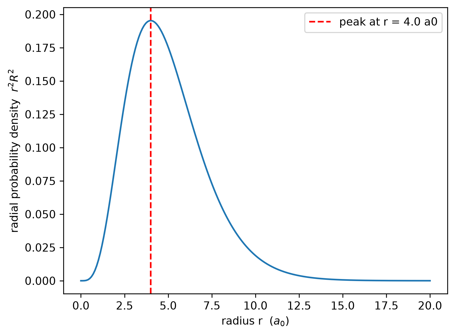

The peak of the $2p$ radial density sits at $r = 4\,a_0$, exactly the Bohr-model radius of the $n = 2$ orbit.

Exercises¶

1. Factor $x^2 + x - 6$.

2. Expand $(x - 2)(x + 5)\,x$.

3. Evaluate $\displaystyle\int_0^{\ln 4} \frac{e^x}{\sqrt{e^{2x} + 9}}\,dx$ with integrate (use log(4) for the upper limit).

4. The reversible isothermal work of a gas is $w = \int_{V_i}^{V_f} -\frac{nRT}{V}\,dV$. Integrate it symbolically, then evaluate for $n = 2.44$ mol, $T = 298$ K, $V_i = 0.552$ L, $V_f = 1.32$ L.

Try it live¶

x = sp.symbols("x")
sp.integrate(sp.sin(x) ** 2, (x, 0, sp.pi))   # try your own integral