DEMO: Linear Variational Method - Quantum Mechanics for Chemistry

Linearizing the problem¶

Basis sets and coefficients

How does linearization help us in practice? If we can not exactly solve and have an expression for $\psi$ then we can expand the wavefunction in some convenient basis set $f_n$ (e.g bunch of functions indexed by n, like fourier series) and attempt to make it get as closer to realistic energies and wavefunction as possible.

\phi(r) = \sum_n^N c_nf_n(r)

(1)

If we have infinite number of basis functions in pricniple that should approximate any funciton and we can get nearly exact numerical solution. However computationally this is not feasible.
Truncating this expansion at any finite $n$ leads to an approximate solution. The idea is to keep just the optimal number of basis functions.
The variational principle tells us is that we can minimize the energy with respect to variational paramters ${c_n}$ and still have $E_\phi \geq E_0$ .

Gaussians are commonly used as basis sets

Gaussian-type orbitals (GTOs) are a standard example because they make integrals analytically tractable. Consider a simple 1s-like primitive Gaussian:

f(r) = e^{-\alpha r^2}

(2)

To represent a more flexible radial shape, we expand the true orbital as a linear combination of Gaussians:

\phi(r) = \sum_{n=1}^N c_n e^{-\alpha_n r^2}

(3)

Even though a hydrogenic 1s orbital behaves as $e^{-r/a_0}$ , which is not Gaussian, we can approximate its shape remarkably well using only 3 to 6 Gaussians. This is the idea behind the STO-nG basis sets.

Smallest example¶

We will illustrate this idea and the general matrix construction with a simple example of two basis functions ( $N=2$ )

\phi = c_1f_1 + c_2f_2

(4)

There is currently no need to define these functions explicitly so we will leave them as generic functions $f_1$ and $f_2$ . We now solve for the energy

E_\phi = \frac{\langle\phi|\hat{H}|\phi\rangle}{\langle\phi|\phi\rangle} = \frac{\langle c_1f_1 + c_2f_2|\hat{H}|c_1f_1 + c_2f_2 \rangle}{\langle c_1f_1 + c_2f_2|c_1f_1 + c_2f_2 \rangle}

(5)

Express problem in terms of coefficients and matrix elements

Let’s investigate the numerator and denomenator separately. We start with the numerator

\langle c_1f_1 + c_2f_2|\hat{H}|c_1f_1 + c_2f_2 \rangle = \langle c_1f_1|\hat{H}|c_1f_1\rangle + \langle c_1f_1|\hat{H}|c_2f_2\rangle +\langle c_2f_2|\hat{H}|c_1f_1\rangle + \langle c_2f_2|\hat{H}|c_2f_2\rangle

(6)

= c_1^*c_1\langle f_1|\hat{H}|f_1\rangle + c_1^*c_2\langle f_1|\hat{H}|f_2\rangle +c_2^*c_1\langle f_2|\hat{H}|f_1\rangle + c_2^*c_2\langle f_2|\hat{H}|f_2\rangle

(7)

We note that $c_i$ are real and thus $c_1^*c_1=c_1^2$ and $c_1c_2=c_2c_1$ thus

Numerator = c_1^2 \langle f_1|\hat{H}|f_1\rangle + c_1c_2\langle f_1|\hat{H}|f_2\rangle +c_2c_1\langle f_2|\hat{H}|f_1\rangle + c_2^2\langle f_2|\hat{H}|f_2\rangle

(8)

Finally we recognize that since $\hat{H}$ is Hermitian, we have $\langle f_2|\hat{H}|f_1\rangle = \langle f_1|\hat{H}|f_2\rangle$ yielding

Numerator = c_1^2 \langle f_1|\hat{H}|f_1\rangle + 2c_1c_2\langle f_1|\hat{H}|f_2\rangle + c_2^2\langle f_2|\hat{H}|f_2\rangle

(9)

We will refer to the integrals above as matrix elements with, generically, $H_{ij} = \langle f_i|\hat{H}|f_j\rangle$ . We now consider the denominator of the energy equation above and we utilize similar algebra for the numerator to get

\langle c_1f_1 + c_2f_2|c_1f_1 + c_2f_2 \rangle = c_1^2S_{11} + 2c_1c_2S_{12} + c_2^2S_{22}

(10)

S_{ij} = \langle f_i|f_j\rangle

(11)

where $S_{ij}$ is another matrix element but this time referred to as the basis function overlap. Now we have that the energy of the trial wavefunction is

E_\phi = \frac{c_1^2 H_{11} + 2c_1c_2H_{12} + c_2^2H_{22}}{c_1^2S_{11} + 2c_1c_2S_{12} + c_2^2S_{22}}

(12)

$H_{ij} = \langle f_i |\hat{H}|f_j\rangle$ Hamiltonian matrix element expressed in basis of $f$
$S_{ij} = \langle f_i|f_j\rangle$ S matrix element or overlap integral expressed in basis of $f$ . This one measures how similiar $f_i$ is to $f_j$ .

Eigenvalue Problem¶

Since $E_\phi \geq E_0$ for any trial function $\phi$ , we can minimize the energy $E_\phi$ by varying the parameters $c_1$ and $c_2$ .
To minimize with respect to $c_1$ , we differentiate $E_\phi$ with respect to $c_1$ and set the derivative equal to zero:
$\frac{\partial E_\phi}{\partial c_1} = 0 = c_1(H_{11} - ES_{11}) + c_2(H_{12} - ES_{12})$
(13)
Similarly, minimizing with respect to $c_2$ gives:
$\frac{\partial E_\phi}{\partial c_2} = 0 = c_1(H_{12} - ES_{12}) + c_2(H_{22} - ES_{22})$
(14)
These two coupled linear equations can be expressed compactly as a matrix equation:
$\begin{bmatrix} H_{11} - ES_{11} & H_{12} - ES_{12} \\ H_{12} - ES_{12} & H_{22} - ES_{22} \end{bmatrix} \begin{bmatrix} c_1 \\ c_2 \end{bmatrix} = 0$
(15)
The matrix on the left can be rewritten as the difference between two matrices:
$\left(\begin{bmatrix} H_{11} & H_{12} \\ H_{12} & H_{22} \end{bmatrix} - E \begin{bmatrix} S_{11} & S_{12} \\ S_{12} & S_{22} \end{bmatrix} \right) \begin{bmatrix} c_1 \\ c_2 \end{bmatrix} = 0$
(16)
Rearranging, we can write:
$\begin{bmatrix} H_{11} & H_{12} \\ H_{12} & H_{22} \end{bmatrix} \begin{bmatrix} c_1 \\ c_2 \end{bmatrix} = E \begin{bmatrix} S_{11} & S_{12} \\ S_{12} & S_{22} \end{bmatrix} \begin{bmatrix} c_1 \\ c_2 \end{bmatrix}$
(17)
Moving S matrix to left hand side we end up with eigenvector eigenvalue problem:

\begin{bmatrix} S_{11} & S_{12} \\ S_{12} & S_{22} \end{bmatrix}^{-1}\begin{bmatrix} H_{11} & H_{12} \\ H_{12} & H_{22} \end{bmatrix} \begin{bmatrix} c_1 \\ c_2 \end{bmatrix} = E \begin{bmatrix} 1 & 0 \\ 0 & 1 \end{bmatrix} \begin{bmatrix} c_1 \\ c_2 \end{bmatrix}

(18)

Reducing QM to a matrix eigenvalue eigenvector problem

\mathbf{H}\mathbf{c} = E\mathbf{S}\mathbf{c}

(19)

By left-multiplying both sides by $\mathbf{S}^{-1}$ , we transform this into a standard eigenvalue problem:
$\mathbf{S}^{-1}\mathbf{H}\cdot \mathbf{c} = E\mathbf{I} \cdot \mathbf{c}$
(20)
Therefore, the minimum energies correspond to the eigenvalues of $\mathbf{S}^{-1}\mathbf{H}$ , and the variational parameters that minimize the energies are the eigenvectors of $\mathbf{S}^{-1}\mathbf{H}$ .
$\mathbf{H}$ N by N matrix of hamiltonian elements $\langle f_i |\hat{H}|f_j\rangle$
$S$ an N by N matrix of overlap integrals $\langle f_i|f_j\rangle$
$\mathbf{c} = (c_1, c_2, ...)$ vector of N length.
$E$ eigenvalues that can saitsfy this equation. For symmetric matrices one expects to get N possible values!

Solving a matrix eigenvalue eigenvector problem

In the equation

\mathbf{S}^{-1}\mathbf{H}\mathbf{c} = E\mathbf{I}\mathbf{c}

(21)

$\mathbf{I}$ represents the identity matrix. Its role in this context is essential to express the equation as a standard eigenvalue problem.

Eigenvalue Problem Form:
In linear algebra, a standard eigenvalue problem is written as:
$\mathbf{A}\mathbf{v} = \lambda \mathbf{I}\mathbf{v}$
(22)
where:
- $\mathbf{A}$ is a square matrix,
- $\lambda$ is a scalar eigenvalue,
- $\mathbf{I}$ is the identity matrix, and
- $\mathbf{v}$ is the corresponding eigenvector.
The identity matrix $\mathbf{I}$ ensures that $\lambda$ scales the eigenvector $\mathbf{v}$ without altering its direction. The eigenvalue problem is about finding the values of $\lambda$ and their associated $\mathbf{v}$ .
Connecting to $\mathbf{S}^{-1}\mathbf{H}\mathbf{c} = E\mathbf{I}\mathbf{c}$ :
Here, $\mathbf{S}^{-1}\mathbf{H}$ acts as the operator $\mathbf{A}$ in the standard eigenvalue problem.
- $\mathbf{S}^{-1}\mathbf{H}$ is a matrix resulting from left-multiplying $\mathbf{H}$ by the inverse of $\mathbf{S}$ .
- $\mathbf{c}$ represents the eigenvector.
- $E$ is the eigenvalue (corresponding to the energy in the quantum mechanical system).
The identity matrix $\mathbf{I}$ is explicitly included to highlight that $E$ is a scalar multiplying the vector $\mathbf{c}$ . This ensures that the left-hand side (a matrix operation) matches the right-hand side (a scaled vector).
Why $\mathbf{S}^{-1}$ Appears:
Initially, we had:
$\mathbf{H}\mathbf{c} = E\mathbf{S}\mathbf{c}$
(23)
which cannot directly be interpreted as an eigenvalue problem because of the presence of $\mathbf{S}$ (the overlap matrix). To transform this into a standard form, we pre-multiply both sides by $\mathbf{S}^{-1}$ :
$\mathbf{S}^{-1}\mathbf{H}\mathbf{c} = E\mathbf{S}^{-1}\mathbf{S}\mathbf{c}$
(24)
Since $\mathbf{S}^{-1}\mathbf{S} = \mathbf{I}$ , this simplifies to:
$\mathbf{S}^{-1}\mathbf{H}\mathbf{c} = E\mathbf{I}\mathbf{c}$
(25)
How to Interpret This as an Eigenvalue Problem:
The equation now has the form of a standard eigenvalue problem:
$\mathbf{A}\mathbf{v} = \lambda \mathbf{I}\mathbf{v}$
(26)
where:
- $\mathbf{A} = \mathbf{S}^{-1}\mathbf{H}$ is the effective matrix to diagonalize,
- $\lambda = E$ are the eigenvalues, corresponding to the energy levels,
- $\mathbf{v} = \mathbf{c}$ are the eigenvectors, containing the coefficients of the trial wavefunctions.
Physical Interpretation:
Solving the eigenvalue problem $\mathbf{S}^{-1}\mathbf{H}\mathbf{c} = E\mathbf{I}\mathbf{c}$ gives the approximate energies ( $E$ ) of the quantum system as eigenvalues and the corresponding variational parameters ( $\mathbf{c}$ ) as eigenvectors. The identity matrix $\mathbf{I}$ is crucial for preserving the standard form of the eigenvalue problem, ensuring proper mathematical and physical interpretation.

Example: Particle in a Box¶

Let’s consider a free particle in 1D bounded to $0\leq x\leq a$ . The Hamiltonian for such a system is simply the kinetic energy operator

\hat{H} = -\frac{\hbar^2}{2m}\frac{d^2}{dx^2}

(27)

While we can have solved this problem analytically, it will be instructive to see how the variational solution works. We start by approximating $\psi(x)$ as an expansion in two basis functions $f_1=x(a-x)$ and $f_2=x^2(a-x)^2$

\psi(x) \approx c_1x(a-x) + c_2x^2(a-x)^2

(28)

The $c_1$ and $c_2$ are the variational parameters to find them we first construct the Hamiltonian matrix, $\mathbf{H}$ , and the basis function overlap matrix, $\mathbf{S}$ .

H_{ij} = \langle f_i|\hat{H}|f_j\rangle

(29)

S_{ij} = \langle f_i|f_j\rangle

(30)

We will then compute and diagonlize the $\mathbf{S}^{-1}\mathbf{H}$ matrix.

Computing the matrix elements

In this problem, we have two basis functions

f_1(x) = x(a-x)

(31)

and

f_2(x) = x^2(a-x)^2

(32)

now the task of computing matrix elements comes down to forming integrals with these two and carrying out integration

H_{11} = \langle x(a-x)|\hat{H}|x(a-x)\rangle

(33)

= \langle ax|\hat{H}|ax\rangle -\langle ax|\hat{H}|x^2\rangle - \langle x^2|\hat{H}|ax\rangle + \langle x^2|\hat{H}|x^2\rangle

(34)

= -a\langle x|\hat{H}|x^2\rangle + \langle x^2|\hat{H}|x^2\rangle

(35)

where the last equality holds because the second derivative of $x$ with respect to x is zero. Let’s now investigate each of these integrals

\langle x|\hat{H}|x^2\rangle = \int_0^ax \frac{-\hbar^2}{2m}\frac{d^2}{dx^2} x^2dx \\ = \frac{-\hbar^2}{m}\int_0^axdx = \frac{-\hbar^2a^2}{2m}

(36)

Similarly we should get

\langle x^2|\hat{H}|x^2\rangle =\frac{-\hbar^2a^3}{3m}

(37)

Thus

H_{11} = -a\frac{-\hbar^2a^2}{2m} + \frac{-\hbar^2a^3}{3m} = \frac{\hbar^2a^3}{6m}

(38)

H_{22} = \langle x^2(a-x)^2|\hat{H}|x^2(a-x)^2\rangle

(39)

= \langle a^2x^2|\hat{H}|a^2x^2\rangle -2\langle a^2x^2|\hat{H}|2ax^3\rangle + \langle a^2x^2|\hat{H}|x^4\rangle -2\langle ax^3|\hat{H}|a^2x^2\rangle + 4\langle ax^3|\hat{H}|ax^3\rangle -2\langle ax^3|\hat{H}|x^4\rangle + \langle x^4|\hat{H}|a^2x^2\rangle - 2\langle x^4|\hat{H}|ax^3\rangle + \langle x^4|\hat{H}|x^4\rangle

(40)

= \frac{-\hbar^2a^7}{3m} +\frac{3\hbar^2 a^7}{m} - \frac{6\hbar^2 a^7}{5m} +\frac{\hbar^2 a^7}{2m} - \frac{12\hbar^2 a^7}{5m} +\frac{2\hbar^2 a^7}{m} - \frac{\hbar^2 a^7}{5m} + \frac{\hbar^2 a^7}{m} - \frac{6\hbar^2 a^7}{7m}

(41)

= \frac{\hbar^2a^7}{105m}

(42)

H_{12} = H_{21} = \frac{\hbar^2a^5}{30m}

(43)

We can now complete the Hamiltonian matrix, $\mathbf{H}$ ,

\mathbf{H} = \frac{\hbar^2a^3}{m} \begin{bmatrix} \frac{1}{6} & \frac{a^2}{30}\\ \frac{a^2}{30} & \frac{a^4}{105} \end{bmatrix}

(44)

Similarily one could carry out all the integrals for $\mathbf{S}$

\mathbf{S} = \frac{a^5}{10} \begin{bmatrix} \frac{1}{3} & \frac{a^2}{14}\\ \frac{a^2}{14} & \frac{a^4}{63} \end{bmatrix}

(45)

We have obtaind all matrix elements in previous section and are now ready to obtain eigenvalues

\mathbf{H} = \frac{\hbar^2a^3}{m} \begin{bmatrix} \frac{1}{6} & \frac{a^2}{30}\\ \frac{a^2}{30} & \frac{a^4}{105} \end{bmatrix}

(46)

\mathbf{S} = \frac{a^5}{10} \begin{bmatrix} \frac{1}{3} & \frac{a^2}{14}\\ \frac{a^2}{14} & \frac{a^4}{63} \end{bmatrix}

(47)

So we see that the smallest energy in this basis is

E_\phi = 4.9349 \frac{\hbar^2}{m}

(48)

How does this compare to the analytic solution? Plugging in for the ground state, $n=1$ , and $a=1$ we get

E_1 = \frac{\pi^2\hbar^2}{2} \approx 4.9348 \frac{\hbar^2}{m}

(49)

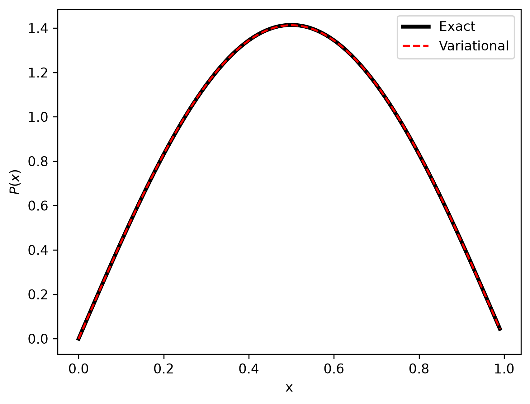
So we can see that our variational solution worked out well for the energy. Now how about the wavefunction?