DEMO: Numerical Schrödinger Solver - Quantum Mechanics for Chemistry

What you need to know

Only a handful of potentials (particle in a box, harmonic oscillator, hydrogen atom) can be solved with pencil and paper. Every other Schrödinger equation in chemistry is solved numerically.
The finite-difference method samples the wavefunction on a grid and replaces derivatives with differences between neighboring points. The Schrödinger equation becomes a matrix eigenvalue problem: eigenvalues are the allowed energies, eigenvectors are the wavefunctions.
Placing a barrier inside a box splits the energy levels into closely spaced tunneling doublets, a first look at a phenomenon that returns in ammonia inversion and hydrogen transfer reactions.
This page is reactive: the Python cells below run live in your browser. Move the slider and every plot that depends on it recomputes. No installation is needed.

From differential equation to matrix problem¶

We want the bound states of the time-independent Schrödinger equation on $0 \le x \le L$ with hard walls, the same boundary conditions as the particle in a box:

-\frac{\hbar^2}{2m}\frac{d^2\psi}{dx^2} + V(x)\,\psi(x) = E\,\psi(x), \qquad \psi(0) = \psi(L) = 0

(1)

Instead of guessing a functional form for $\psi(x)$ , we store its values $\psi_1, \psi_2, \dots, \psi_N$ at $N$ evenly spaced grid points, as sketched in Figure 1. On the grid, the second derivative at point $j$ is approximated by the classic three-point formula Press et al., 2007:

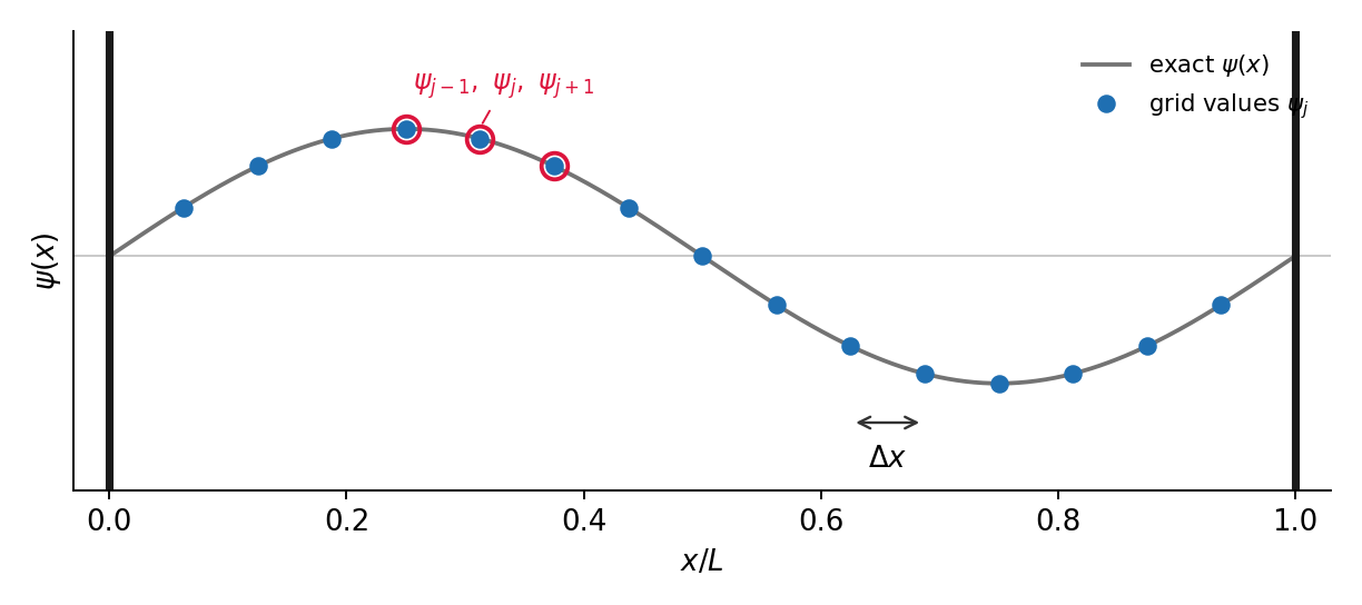
\frac{d^2\psi}{dx^2}\bigg|_{x_j} \approx \frac{\psi_{j+1} - 2\psi_j + \psi_{j-1}}{\Delta x^2}

(2)

A smooth wavefunction sampled at evenly spaced grid points between two hard walls — Figure 1:A wavefunction sampled on a uniform grid between hard walls. The curvature at point $j$ is built from the point and its two neighbors (red circles), which turns the differential equation into a matrix problem.

Substituting (2) into (1) gives one linear equation per grid point. Collecting them produces a matrix eigenvalue problem $\mathbf{H}\,\boldsymbol{\psi} = E\,\boldsymbol{\psi}$ with a tridiagonal Hamiltonian: kinetic energy couples each point only to its two neighbors, and the potential sits on the diagonal.

\mathbf{H} = \frac{\hbar^2}{2m\,\Delta x^2} \begin{pmatrix} 2 & -1 & & \\ -1 & 2 & -1 & \\ & \ddots & \ddots & \ddots \\ & & -1 & 2 \end{pmatrix} + \begin{pmatrix} V_1 & & & \\ & V_2 & & \\ & & \ddots & \\ & & & V_N \end{pmatrix}

(3)

Diagonalizing $\mathbf{H}$ hands us energies and wavefunctions in one shot. The LAPACK routines that do this are the same machinery running inside every modern quantum chemistry package.

A box with a barrier inside¶

As a test system we take the unit box and drop a rectangular barrier of height $V_0$ and width $L/4$ into the middle. With $\hbar = m = L = 1$ , the natural energy unit is the ground-state energy of the empty box from the particle in a box lecture:

E_1 = \frac{\pi^2 \hbar^2}{2mL^2} = \frac{h^2}{8mL^2}

(4)

For $V_0 = 0$ the solver must reproduce $E_n = n^2 E_1$ exactly, which is a good sanity check. As $V_0$ grows, the box splits into two weakly coupled half-boxes, and pairs of levels squeeze together into doublets: a symmetric state with no node at the center and an antisymmetric partner with one. Their tiny energy difference is the tunneling splitting, the standard textbook route to double-well physics Griffiths & Schroeter, 2018.

The live solver¶

We need only the course’s standard scientific stack: NumPy for arrays, SciPy for the tridiagonal eigensolver, and Matplotlib for plots.

The solver builds the two diagonals of $\mathbf{H}$ and asks SciPy for the lowest few eigenpairs. Dividing the eigenvectors by $\sqrt{\Delta x}$ normalizes them so that $\int |\psi|^2\,dx = 1$ .

Drag the slider to raise or lower the barrier. Everything below it reacts.

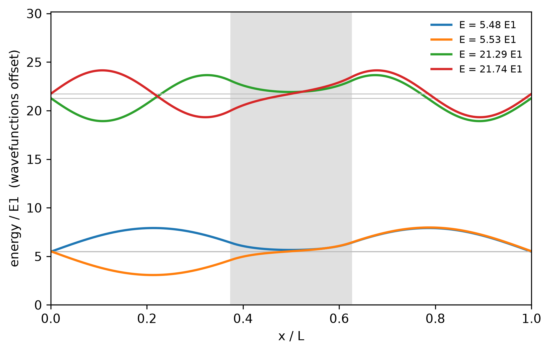
With the barrier at zero you should read off $E/E_1 = 1, 4, 9, 16$ , the exact particle in a box ladder. Raise the barrier and watch $n = 1, 2$ collapse onto each other while keeping opposite symmetry about the center.

Tunneling doublets across all barrier heights¶

A single click of the slider solves one Hamiltonian. The cell below instead sweeps the full range of barrier heights, a moderately expensive computation: 51 diagonalizations of a $2000 \times 2000$ matrix, tracking the six lowest states. Because it does not read the slider, marimo executes it once and reuses the cached result no matter how much you play with the plots.

The correlation diagram replots instantly when you move the slider, because only the cheap plotting cell reruns, not the sweep.

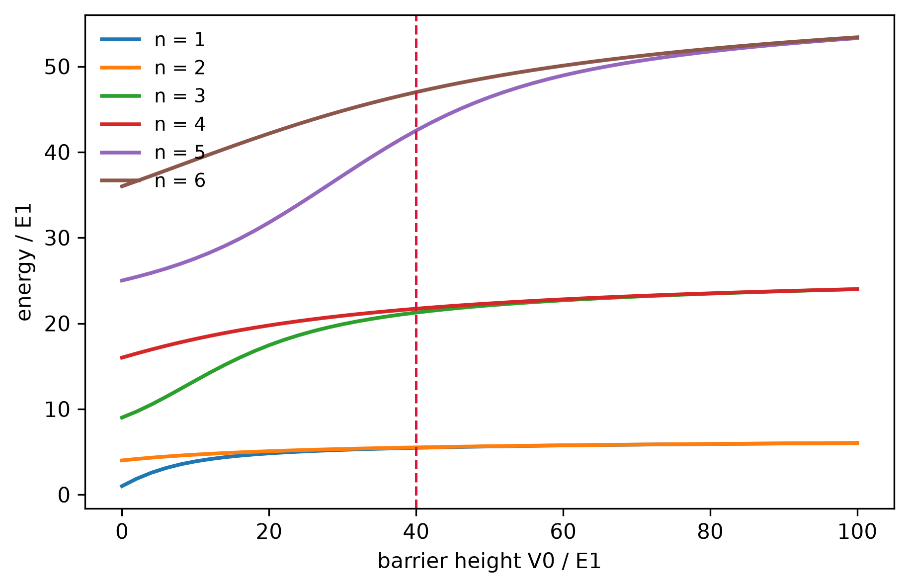
How this page works

This demo pilots marimo cells inside the course website. The cells are executed while the site is built, so the page loads with correct static output. The first time you touch the slider, a Python runtime (Pyodide, Python compiled to WebAssembly) downloads in the background along with NumPy, SciPy, and Matplotlib, and from then on all cells rerun locally in your browser. Unlike the ipywidgets demos, nothing needs to run on a server, and unlike static pages, every plot stays live.

References¶

Press, W. H., Teukolsky, S. A., Vetterling, W. T., & Flannery, B. P. (2007). Numerical Recipes: The Art of Scientific Computing (3rd ed.). Cambridge University Press.
Griffiths, D. J., & Schroeter, D. F. (2018). Introduction to Quantum Mechanics (3rd ed.). Cambridge University Press. 10.1017/9781316995433