Setting up the Hamiltonian
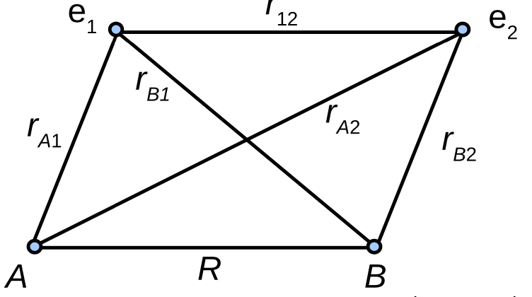
Fig. 1 Coordinates used to describe the two electrons and two nuclei of the molecule.
The main difficulty in the molecular Hamiltonian is the term, which couples the two electrons to each other. This means that a simple product wavefunction is not sufficient. No analytic solution has been found for the electronic Schrodinger equation of .
For this reason, we solve the problem approximately by using the LCAO-MO approach used previously. For example, the ground state for is obtained by placing two electrons with opposite spins in the orbital. This assumes that the wavefunction is expressed as an antisymmetrized product (a Slater determinant).
Constructing MOs for the hydrogen molecule
According to the Pauli principle, two electrons with opposite spins can be assigned to a given spatial orbital. As a first approximation, we assume that the molecular orbitals in remain the same as in . Hence both electrons occupy the orbital (the ground state) and the electronic configuration is denoted (. This is similar to the notation used previously for atoms (for example, the He atom is ().
The molecular orbital for electron 1 in the molecular orbital is:
Previously we found that the total wavefunction must be antisymmetric with respect to exchange of electron indices. This can be achieved by using the Slater determinant:
where and denote the electron spin. The Slater determinant can be expanded as follows:
Note that this wavefunction is only approximate and is definitely not an eigenfunction of the electronic Hamiltonian. Thus we must calculate the electronic energy by taking the expectation value of this wavefunction with the Hamiltonian (the actual calculation is not shown):
where is the electronic energy of one hydrogen atom. The second term represents the Coulomb repulsion between the two positively charged nuclei, and the last term (“integrals”) contains a series of integrals describing the interactions of various charge distributions with one another (see P. W. Atkins, Molecular Quantum Mechanics, Oxford University Press). With this approach, the minimum energy is reached at = 84 pm (experimental 74.1 pm) with a dissociation energy = 255 kJ mol (experimental 458 kJ mol).
Improving upon the simple MO approximation
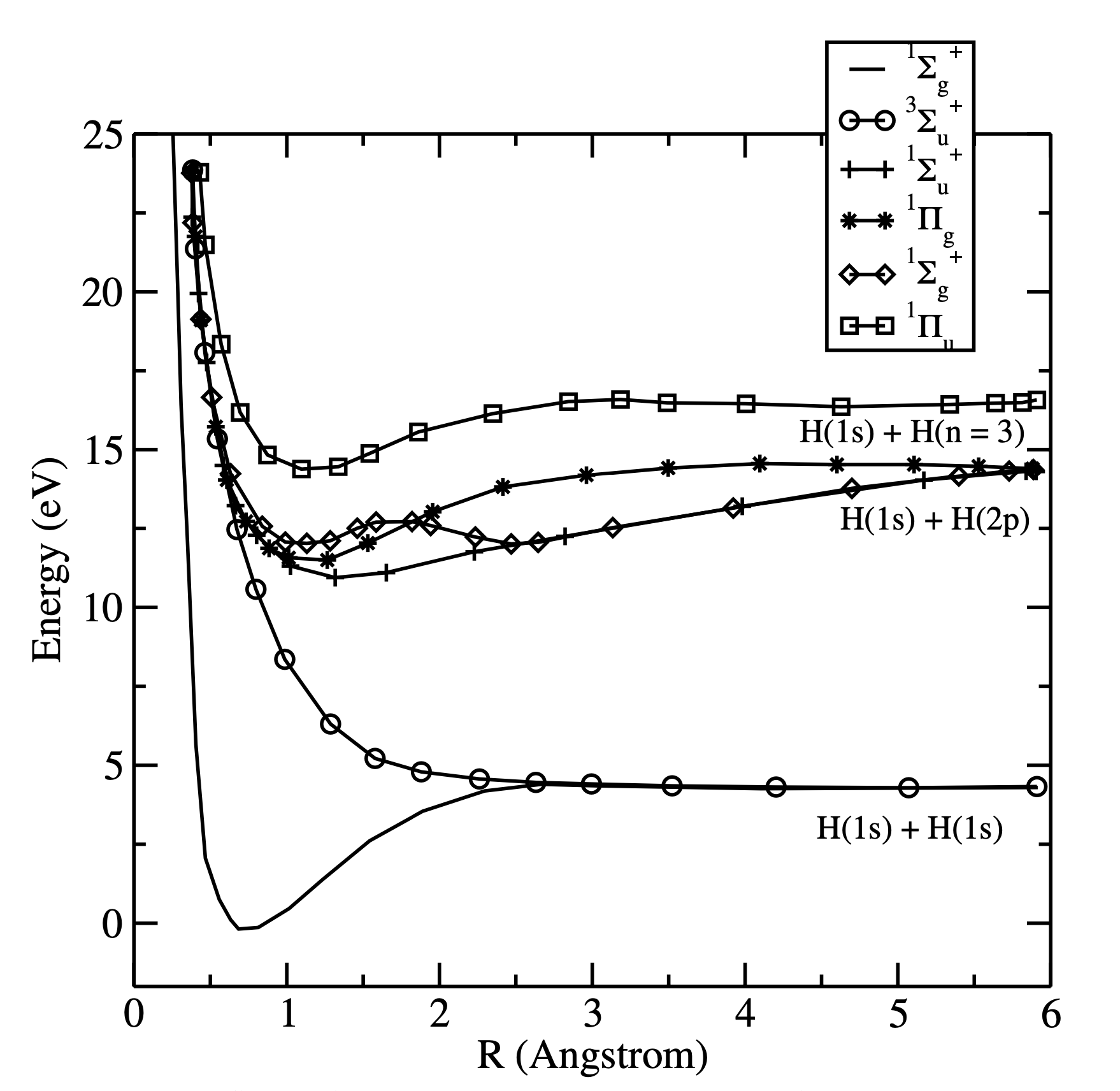
Fig. 2 Improving the wavefunction by treating ionic and covalent contributions separately lowers the energy and shortens the predicted bond length toward experiment.
This simple approach is not very accurate, but it demonstrates that the method works. To improve the accuracy, ionic and covalent terms should be considered separately:
Both covalent and ionic terms can be introduced into the wavefunction with their own variational parameters and :
Note that the variational constants and depend on the internuclear distance . Minimization of the energy expectation value with respect to these constants gives = 74.9 pm (experiment 74.1 pm) and = 386 kJ mol (experiment 458 kJ mol).
Further improvement can be achieved by adding higher atomic orbitals to the wavefunction. The previously discussed Hartree-Fock method provides an efficient way of solving the problem. Recall that this method is only approximate, as it ignores electron-electron correlation effects completely. The full treatment requires configuration interaction methods, which can yield essentially exact results: = 36117.8 cm (CI) versus cm (experiment), and = 74.140 pm versus 74.139 pm (experiment).