The Hydrogen Molecule Ion - Quantum Mechanics for Chemistry

Constructing MOs from AOs¶

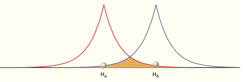
1s atomic orbitals centered on each hydrogen atom — Fig. 1 The 1s atomic orbitals centered on each H atom in the $H_2^+$ molecule.

The electronic Schrodinger equation for $H_2^+$ can be solved exactly because the system contains only a single electron. However, the analytical solution involves quite challenging mathematics. Instead, we adopt a simpler approximate approach that still captures the essential physics of chemical bonding.

We construct a trial (approximate) molecular wavefunction as a real linear combination of hydrogen 1s atomic orbitals:

\psi_{\pm}(\vec{r}_1) = c_1\,1s_A(\vec{r}_1) \; \pm \; c_2\,1s_B(\vec{r}_1)

(1)

Here, $1s_A$ and $1s_B$ are hydrogen 1s orbitals centered on nuclei A and B, respectively, and $c_1$ and $c_2$ are coefficients (constants).
This form is known as the Linear Combination of Atomic Orbitals (LCAO) approximation for constructing molecular orbitals.
Because the two nuclei are identical, symmetry requires $c_1 = c_2 \equiv c$ (and we choose $c > 0$ ).
The ± sign indicates that two distinct molecular orbitals can be formed:
- the bonding combination ( $+$ ), which enhances electron density between the nuclei
- the antibonding combination ( $-$ ), which decreases electron density between the nuclei
Normalization of the molecular wavefunction requires:

{\int{\psi_\pm^*\psi_\pm d\tau} = 1}

(2)

The overlap integral¶

We now consider the bonding molecular orbital (the “+” combination) and evaluate the normalization condition.
Here, $S$ is the overlap integral, which depends on the internuclear distance $R$ :

1 = \int |\psi_+|^2 \, d\tau = c^2 \int (1s_A + 1s_B)(1s_A + 1s_B) \, d\tau

(3)

Expanding the integrand:

\begin{aligned} 1 &= c^2 \int \left(1s_A^2 + 1s_B^2 + 2\,1s_A\,1s_B \right) d\tau \\ &= c^2 \left( \int 1s_A^2 d\tau + \int 1s_B^2 d\tau + 2\int 1s_A\,1s_B\, d\tau \right) \end{aligned}

(4)

Normalized atomic orbitals satisfy:

\int 1s_A^2 d\tau = \int 1s_B^2 d\tau = 1

(5)

Defining the overlap integral:

S = \int 1s_A(\vec{r})\,1s_B(\vec{r})\, d\tau

(6)

we obtain:

1 = c^2(2 + 2S) \quad \Rightarrow \quad c = \frac{1}{\sqrt{2(1 + S)}}

(7)

Bonding versus antibonding orbitals¶

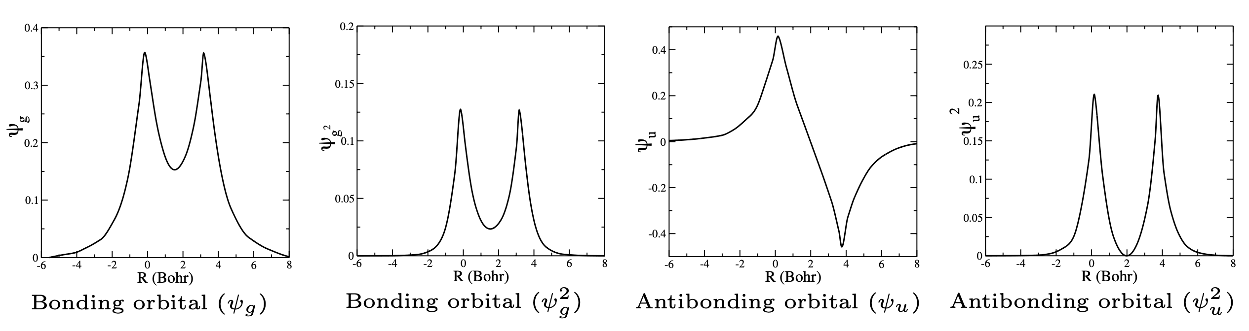
Bonding versus antibonding wavefunctions and densities — Fig. 2 Bonding versus antibonding wavefunctions (molecular orbitals). Shown are the wavefunctions and the probability densities (squares of the wavefunctions).

The main feature of a chemical bond is the increased electron density between the nuclei. This identifies the $+$ wavefunction as a bonding orbital and the $-$ wavefunction as an antibonding orbital.
When a molecule has a center of symmetry (here halfway between the nuclei), the wavefunction may or may not change sign when it is inverted through the center of symmetry. If the origin is placed at the center of symmetry, then we can assign symmetry labels $g$ and $u$ to the wavefunctions.
If $\psi(x, y, z) = \psi(-x, -y, -z)$ then the symmetry label is $g$ (even parity), and for $\psi(x, y, z) = -\psi(-x, -y, -z)$ we have the $u$ label (odd parity).
According to this notation, the $g$ symmetry orbital is the bonding orbital and the $u$ symmetry corresponds to the antibonding orbital. Later we will see that this is reversed for $\pi$ -orbitals.
The overlap integral $S(R)$ can be evaluated analytically (derivation not shown):

{S(R) = e^{-R}\left( 1 + R + \frac{R^3}{3}\right)}

(10)

Note that when $R = 0$ (the nuclei overlap), $S(0) = 1$ , which is a useful check that the expression is reasonable.

Energy of the hydrogen molecule ion¶

Using a linear combination of atomic orbitals, it is possible to calculate the best values, in terms of energy, of the coefficients $c_1$ and $c_2$ . Remember that this linear combination can only provide an approximate solution to the $H_2^+$ Schrodinger equation. The variational principle provides a systematic way to calculate the energy when $R$ (the distance between the nuclei) is fixed:

{E = \frac{\int\psi_g^*\hat{H}_e\psi_gd\tau}{\int\psi_g^*\psi_gd\tau} = \frac{\int (c_11s_A + c_21s_B)\hat{H}_e(c_11s_A + c_21s_B)d\tau} {\int (c_11s_A + c_21s_B)^2d\tau}}

(11)

{= \frac{c_1^2H_{AA} + 2c_1c_2H_{AB} + c_2^2H_{BB}} {c_1^2 S_{AA} + 2c_1c_2 S_{AB} + c_2^2 S_{BB}}}

(12)

where $S_{AA} = S_{BB} = 1$ and $S_{AB} = S$ .

Here $H_{AA}$ , $H_{AB}$ , $H_{BB}$ , $S_{AA}$ , $S_{AB}$ , and $S_{BB}$ denote the integrals occurring in the variational treatment of the problem. The integrals $H_{AA}$ and $H_{BB}$ are called the Coulomb integrals (sometimes more generally termed matrix elements).
This interaction is attractive, and therefore its numerical value must be negative. Note that by symmetry $H_{AA} = H_{BB}$ . The integral $H_{AB}$ is called the resonance integral, and also by symmetry $H_{AB} = H_{BA}$ .

Variational solution¶

To minimize the energy expectation value with respect to $c_1$ and $c_2$ , we calculate the partial derivatives of the energy with respect to these parameters:

{E\times (c_1^2 + 2c_1c_2S + c_2^2) = c_1^2H_{AA} + 2c_1c_2H_{AB} + c_2^2H_{BB}}

(13)

Both sides can be differentiated with respect to $c_1$ to give:

{E\times (2c_1 + 2c_2S) + \frac{\partial E}{\partial c_1}\times (c_1^2 + 2c_1c_2S + c_2^2) = 2c_1H_{AA} + 2c_2H_{AB}}

(14)

In a similar way, differentiation with respect to $c_2$ gives:

{E\times (2c_2 + 2c_1S) + \frac{\partial E}{\partial c_2}\times (c_1^2 + 2c_1c_2S + c_2^2) = 2c_2H_{BB} + 2c_1H_{AB}}

(15)

At the minimum energy (with respect to $c_1$ and $c_2$ ), the partial derivatives must be zero:

{c_1(H_{AA} - E) + c_2(H_{AB} - SE) = 0}

(16)

{c_2(H_{BB} - E) + c_1(H_{AB} - SE) = 0}

(17)

In matrix notation this is a generalized matrix eigenvalue problem:

{\begin{pmatrix}H_{AA} - E & H_{AB} - SE\\ H_{AB} - SE & H_{BB} - E\\ \end{pmatrix}\begin{pmatrix} c_1\\ c_2\\\end{pmatrix} = 0}

(18)

From linear algebra, we know that a non-trivial solution exists only if the secular determinant vanishes:

{\begin{vmatrix}H_{AA} - E & H_{AB} - SE\\ H_{AB} - SE & H_{BB} - E\\ \end{vmatrix} = 0}

(19)

Energies of the bonding and antibonding orbitals¶

It can be shown that $H_{AA} = H_{BB} = E_{1s} + J(R)$ , where $E_{1s}$ is the energy of a single hydrogen atom and $J(R)$ is a function of the internuclear distance $R$ :

{J(R) = e^{-2R}\left( 1 + \frac{1}{R}\right)}

(20)

Furthermore, $H_{AB} = H_{BA} = E_{1s}S(R) + K(R)$ , where $K(R)$ is also a function of $R$ :

{K(R) = \frac{S(R)}{R} - e^{-R}\left( 1 + R\right)}

(21)

If these expressions are substituted into the previous secular determinant, we get:

{\begin{vmatrix}E_{1s} + J - E & E_{1s}S + K - SE\\ E_{1s}S + K - SE & E_{1s} + J - E\\ \end{vmatrix} = (E_{1s} + J - E)^2 - (E_{1s}S + K - SE)^2 = 0}

(22)

This equation has two roots:

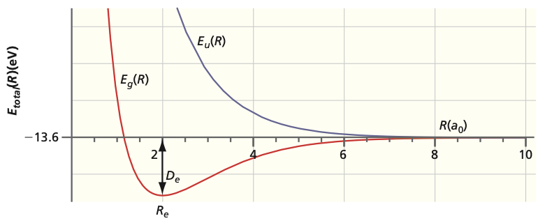
Energies of bonding and antibonding orbitals — Fig. 3 Energies of the bonding and antibonding orbitals as a function of internuclear distance.

Since energy is a relative quantity, it can be expressed relative to the separated nuclei:

{\Delta E_g(R) = E_g(R) - E_{1s} = \frac{J(R) + K(R)}{1 + S(R)}}

(25)

{\Delta E_u(R) = E_u(R) - E_{1s} = \frac{J(R) - K(R)}{1 - S(R)}}

(26)

Comparison of MO energies with experiment¶

These values can be compared with experimental results. The calculated ground state equilibrium bond length is 132 pm, whereas the experimental value is 106 pm. The binding energy is 170 kJ mol $^{-1}$ , whereas the experimental value is 258 kJ mol $^{-1}$ .
The excited state (labeled with $u$ ) leads to repulsive behavior at all bond lengths $R$ (it is antibonding). Because the $u$ state lies higher in energy than the $g$ state, the $u$ state is an excited state of $H_2^+$ .
This calculation can be made more accurate by adding more than two terms to the linear combination. This procedure would also yield more excited state solutions. These would correspond to $u$ / $g$ combinations of $2s$ , $2p_x$ , $2p_y$ , $2p_z$ , and so on.

MO diagrams¶

It is common practice to represent the molecular orbitals using molecular orbital (MO) diagrams. The formation of bonding and antibonding orbitals can be visualized as follows:

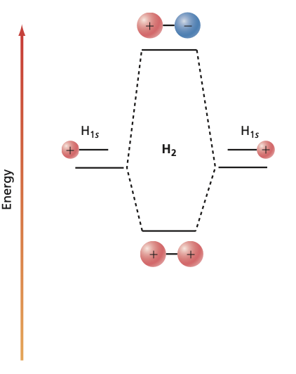
Molecular orbital diagram for the hydrogen molecule ion — Fig. 4 Molecular orbital diagram for $H_2^+$ .

$\sigma$ orbitals. When two $s$ or $p_z$ orbitals interact, a $\sigma$ molecular orbital is formed. The notation $\sigma$ specifies the amount of angular momentum about the molecular axis (for $\sigma$ , $\lambda = 0$ with $L_z = \pm\lambda\hbar$ ). In many-electron systems, both bonding and antibonding $\sigma$ orbitals can each hold a maximum of two electrons. Antibonding orbitals are often denoted by an asterisk.

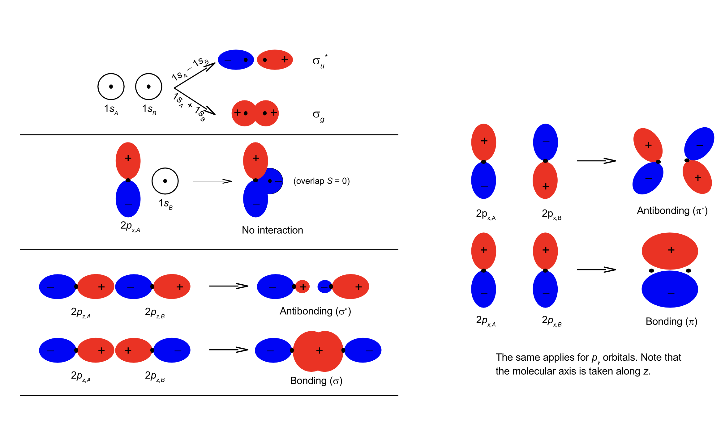
Molecular orbitals for homonuclear molecules — Fig. 5 MOs for homonuclear molecules have distinct symmetry.

$\pi$ orbitals. When two $p_{x,y}$ orbitals interact, a $\pi$ molecular orbital forms. $\pi$ -orbitals are doubly degenerate: $\pi_{+1}$ and $\pi_{-1}$ (or alternatively $\pi_x$ and $\pi_y$ ), where the $+1/-1$ refer to the eigenvalue of the $L_z$ operator ( $\lambda = \pm1$ ). In many-electron systems a bonding $\pi$ -orbital can therefore hold a maximum of 4 electrons (both $\pi_{+1}$ and $\pi_{-1}$ each hold two electrons). The same holds for the antibonding $\pi$ orbitals. Note that only atomic orbitals of the same symmetry mix to form molecular orbitals (for example, $p_z - p_z$ , $p_x - p_x$ , and $p_y - p_y$ ). 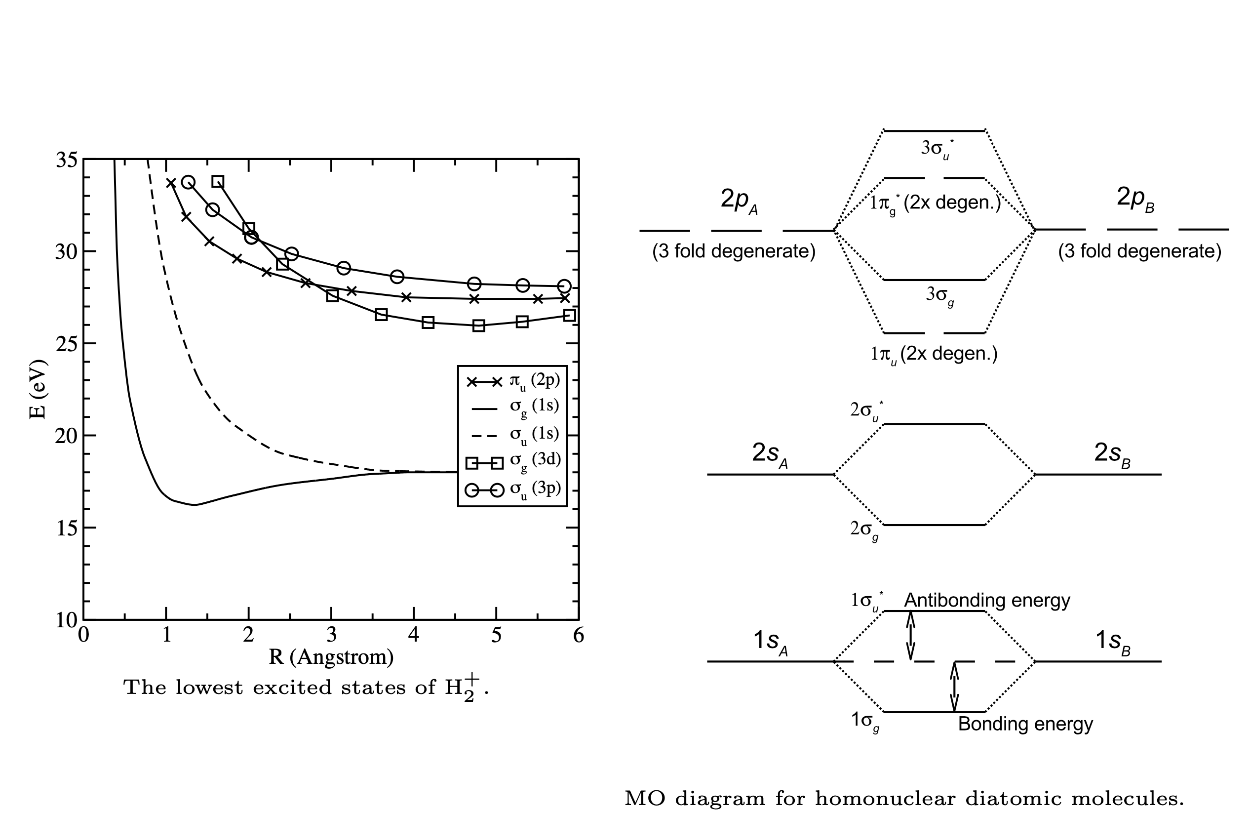When atomic $d$ orbitals mix to form molecular orbitals, $\sigma$ ( $\lambda = 0$ ), $\pi$ ( $\lambda = \pm 1$ ), and $\delta$ ( $\lambda = \pm 2$ ) MOs form.

Fig. 6 The MO diagram of homonuclear molecules follows a similar pattern with alternating bonding and antibonding MOs.

Excited state energies of $H_2^+$ resulting from a calculation employing an extended basis set (more terms in the LCAO) are shown on the left below. The MO energy diagram, which includes the higher energy molecular orbitals, is shown on the right. Note that the energy order of the MOs depends on the molecule.