Operators and Differential Equations - Quantum Mechanics for Chemistry

Quantum mechanics is written in the language of operators and differential equations. But underneath that calculus lies a simpler and more powerful truth: quantum mechanics is linear algebra. Wavefunctions are vectors, operators are matrices, and the Schrodinger equation is the eigenvalue problem $A\mathbf{v} = \lambda\mathbf{v}$ in disguise. Undergraduate courses often bury this under derivatives and integrals; this page brings it to the surface first, then returns to the differential equations as the tools for working in one particular basis.

Functions are vectors, operators are matrices¶

A function is a vector with one component per point¶

Take any function and evaluate it at $N$ points $x = (x_1, x_2, \ldots, x_N)$ . The list of values is a vector with $N$ components. For example $f(x) = x^2$ sampled at $x = (0,1,2,3,4)$ becomes the vector $(0,1,4,9,16)$ .

Now let the grid get finer, $N\to\infty$ with spacing $h\to 0$ . The vector gains a component for every point $x$ , and in that limit the function is an infinite-dimensional vector. The value $\psi(x)$ plays the role of “the component at $x$ ,” exactly as $v_i$ is the component of $\mathbf{v}$ along basis direction $i$ .

The inner product becomes an integral¶

This is the link that makes the analogy precise. The dot product of two vectors sums the products of matching components. For function-vectors, that sum over grid points, weighted by the spacing $h$ , is a Riemann sum, and in the fine-grid limit it becomes an integral:

\langle f \mid g \rangle = \sum_i f^*(x_i)\,g(x_i)\,h \;\xrightarrow[h\to 0]{}\; \int f^*(x)\,g(x)\,dx.

(1)

So the quantum-mechanical inner product $\langle\psi\mid\phi\rangle = \int\psi^*\phi\,dx$ is nothing more than the dot product from the previous page, carried to infinite dimensions. Everything built on the dot product carries over verbatim: normalization $\int|\psi|^2\,dx = 1$ is just $|\psi| = 1$ , and orthogonal wavefunctions ( $\int\psi_m^*\psi_n\,dx = 0$ ) are just perpendicular vectors.

An operator is a matrix¶

A linear operator takes a function and returns a function, that is, it takes a vector and returns a vector. Any linear map on vectors is a matrix, so every quantum operator is a matrix acting on the function-vector. The derivative operator, for instance, becomes the finite-difference matrix built in the next section. This gives the full dictionary between the linear algebra you already know and the quantum mechanics ahead:

Linear algebra (finite dimensions)	Quantum mechanics (functions)
vector $\mathbf{v}$	wavefunction $\psi(x)$
component $v_i$	value $\psi(x)$
dot product $\langle \mathbf{a}\mid\mathbf{b}\rangle = \sum_i a_i^* b_i$	inner product $\langle\psi\mid\phi\rangle = \int\psi^*\phi\,dx$
normalized $\lvert\mathbf{v}\rvert = 1$	normalized $\int\lvert\psi\rvert^2 dx = 1$
orthonormal basis $\mathbf{e}_i$	orthonormal functions $\phi_n(x)$
matrix $A$	operator $\hat A$ (such as $\hat x$ , $\hat p$ , $\hat H$ )
eigenvector equation $A\mathbf{v} = \lambda\mathbf{v}$	eigenfunction equation $\hat A\psi = a\psi$
eigenvalue $\lambda$	measured value $a$ (energy, momentum)
symmetric / Hermitian matrix	Hermitian operator (real eigenvalues)
expansion $\mathbf{v} = \sum_i c_i\mathbf{e}_i$	superposition $\psi = \sum_n c_n\phi_n$

The rest of this page makes the “operator is a matrix” half concrete: we build the derivative as an explicit matrix, see why operator order matters, and then meet the differential equations that these operators live in.

The derivative as a finite-difference matrix¶

We approximate the first derivative by a centered difference, the slope between the neighbor on the left and the neighbor on the right:

\frac{d\psi}{dx}\bigg|_{x_i} \approx \frac{\psi(x_{i+1}) - \psi(x_{i-1})}{2h}.

(2)

Written as a matrix acting on the sampled vector (with one-sided formulas at the two boundaries), this is

D_1 = \frac{1}{2h} \begin{pmatrix} -3 & 4 & -1 & 0 & 0 \\ -1 & 0 & 1 & 0 & 0 \\ 0 & -1 & 0 & 1 & 0 \\ 0 & 0 & -1 & 0 & 1 \\ 0 & 0 & 1 & -4 & 3 \end{pmatrix}.

(3)

import numpy as np

n = 5
x = np.linspace(0, 4, n)
h = x[1] - x[0]
psi = x**2

D1 = (1 / (2 * h)) * np.array([
    [-3, 4, -1, 0, 0],
    [-1, 0, 1, 0, 0],
    [0, -1, 0, 1, 0],
    [0, 0, -1, 0, 1],
    [0, 0, 1, -4, 3],
])

print("finite-difference derivative of x^2:", D1 @ psi)
print("exact derivative 2x               :", 2 * x)

finite-difference derivative of x^2: [0. 2. 4. 6. 8.]
exact derivative 2x               : [0. 2. 4. 6. 8.]

The second derivative uses the three-point stencil $\psi_{i+1} - 2\psi_i + \psi_{i-1}$ over $h^2$ . This matrix is the discrete kinetic-energy operator, the heart of every numerical Schrodinger solver. Below we build it on a fine grid, apply it to $\sin x$ , and recover $-\sin x$ , since $\frac{d^2}{dx^2}\sin x = -\sin x$ .

import numpy as np
import matplotlib.pyplot as plt

N = 200
x = np.linspace(0, 2 * np.pi, N)
h = x[1] - x[0]

# Second-derivative matrix, tridiagonal (1, -2, 1) / h^2
D2 = (np.diag(np.ones(N - 1), 1)
      - 2 * np.diag(np.ones(N))
      + np.diag(np.ones(N - 1), -1)) / h**2

psi = np.sin(x)
d2psi = D2 @ psi

fig, ax = plt.subplots(figsize=(7, 3.6))
ax.plot(x, psi, 'k', lw=2, label=r'$\psi = \sin x$')
ax.plot(x[1:-1], d2psi[1:-1], color='#d1495b', lw=2, label=r'$D_2\,\psi$ (numerical)')
ax.plot(x, -np.sin(x), '--', color='#66a182', lw=2, label=r'$-\sin x$ (exact)')
ax.axhline(0, color='gray', lw=0.6)
ax.set_xlabel('x')
ax.legend(fontsize=9, loc='upper right')
ax.set_title('Fig.1 The second-derivative matrix turns sin x into -sin x')
plt.tight_layout()
plt.show()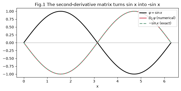

Operator order matters¶

Matrices, and therefore operators, generally do not commute: $AB \neq BA$ . With

A = \begin{pmatrix} 1 & 2 \\ 0 & 1 \end{pmatrix}, \qquad B = \begin{pmatrix} 0 & 1 \\ 1 & 0 \end{pmatrix},

(4)

we get $AB = \begin{pmatrix} 2 & 1 \\ 1 & 0 \end{pmatrix}$ but $BA = \begin{pmatrix} 0 & 1 \\ 1 & 2 \end{pmatrix}$ .

import numpy as np

A = np.array([[1, 2], [0, 1]])
B = np.array([[0, 1], [1, 0]])

print("AB =\n", A @ B)
print("BA =\n", B @ A)
print("\ncommutator AB - BA =\n", A @ B - B @ A)

AB =
 [[2 1]
 [1 0]]
BA =
 [[0 1]
 [1 2]]

commutator AB - BA =
 [[ 2  0]
 [ 0 -2]]

The order matters because applying a shear then a rotation is not the same as rotation then shear. In quantum mechanics this same non-commutation, packaged as the commutator $[\hat A, \hat B] = \hat A\hat B - \hat B\hat A$ , is exactly what forbids simultaneous sharp values of position and momentum. It is the algebra behind the uncertainty principle.

When do operators commute?

Diagonal matrices always commute with each other, and the identity commutes with everything. More generally, two operators commute if and only if they share a common set of eigenvectors, which is the condition for two observables to be simultaneously measurable.

Ordinary differential equations¶

A differential equation relates a function to its derivatives. An ordinary differential equation (ODE) involves derivatives with respect to a single variable. Two show up everywhere in chemistry.

First order: exponential growth and decay¶

The rate of change is proportional to the amount present. With $k < 0$ this is radioactive decay or a first-order reaction; with $k > 0$ it is unchecked growth. The solution is the exponential because $e^{kt}$ is the one function equal to its own derivative up to the constant $k$ .

Second order: oscillation¶

Here the second derivative is proportional to the negative of the function, so the solution oscillates. This is a swinging pendulum, a vibrating bond, and, with $x$ in place of $t$ , the spatial shape of a particle-in-a-box wavefunction. Using Euler’s formula the same solution reads $y = C e^{i\omega t} + D e^{-i\omega t}$ , which is why complex exponentials and oscillations are inseparable.

import numpy as np
import matplotlib.pyplot as plt

t = np.linspace(0, 10, 400)

fig, axes = plt.subplots(1, 2, figsize=(10, 3.6))

# First order: decay for several rates
for k, c in zip([-0.2, -0.5, -1.0], ['#66a182', '#edae49', '#d1495b']):
    axes[0].plot(t, np.exp(k * t), color=c, lw=2, label=f'k = {k}')
axes[0].set_title(r"Fig.2a First order: $y' = ky$ (decay)")
axes[0].set_xlabel('t')
axes[0].set_ylabel('y')
axes[0].legend(fontsize=9)

# Second order: oscillation for several frequencies
for w, c in zip([1.0, 1.5, 2.0], ['#66a182', '#edae49', '#d1495b']):
    axes[1].plot(t, np.cos(w * t), color=c, lw=2, label=fr'$\omega$ = {w}')
axes[1].set_title(r"Fig.2b Second order: $y'' = -\omega^2 y$ (oscillation)")
axes[1].set_xlabel('t')
axes[1].axhline(0, color='gray', lw=0.6)
axes[1].legend(fontsize=9)

plt.tight_layout()
plt.show()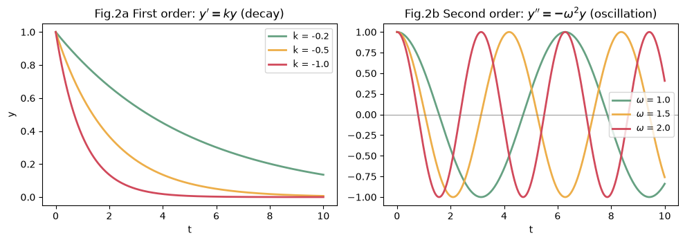

Partial differential equations¶

A partial differential equation (PDE) involves derivatives with respect to more than one variable, for example both position $x$ and time $t$ . The two central equations of the course are PDEs:

\text{Wave equation:}\quad \frac{\partial^2 u}{\partial t^2} = c^2\frac{\partial^2 u}{\partial x^2}, \qquad \text{Schrodinger:}\quad i\hbar\frac{\partial \Psi}{\partial t} = \hat H \Psi.

(7)

Separation of variables¶

The workhorse technique is separation of variables: guess that the solution factors into pieces that each depend on only one variable,

\Psi(x, t) = \psi(x)\,T(t).

(8)

Substituting this guess turns one PDE into two independent ODEs, one in $x$ and one in $t$ , tied together by a shared constant. For the Schrodinger equation the spatial ODE is the time-independent Schrodinger equation $\hat H \psi = E\psi$ , and the temporal ODE gives the phase factor $T(t) = e^{-iEt/\hbar}$ .

This is why the earlier ODE solutions matter: the spatial equation is a second-order ODE whose oscillating solutions are the stationary states, and the temporal equation is a first-order ODE whose solution is a complex-exponential phase. Notice the recurring pattern of the whole appendix: the eigenvalue problem $\hat H\psi = E\psi$ is the operator-as-matrix idea, the energies $E$ are eigenvalues, and the wavefunctions $\psi$ are eigenvectors.

Problems¶

Problem 1: Read off a derivative matrix¶

Using the first-derivative matrix $D_1$ above with $h=1$ , apply it to the constant vector $\psi = (5,5,5,5,5)$ . What do you expect, and why?

Solution

Each interior row computes a difference of equal neighbors, so the derivative is 0 everywhere. The derivative of a constant is zero, and the boundary rows are built to return zero for a constant as well.

Problem 2: Solve a decay ODE¶

A first-order reaction obeys $dy/dt = -0.3\,y$ with $y_0 = 2$ . Write $y(t)$ and find the half-life.

Solution

y(t) = 2\,e^{-0.3 t}.

(9)

The half-life solves $e^{-0.3 t_{1/2}} = \tfrac{1}{2}$ , giving $t_{1/2} = \dfrac{\ln 2}{0.3} \approx 2.31$ .

Problem 3: Verify an oscillator solution¶

Show that $y(t) = A\cos(\omega t) + B\sin(\omega t)$ satisfies $y'' = -\omega^2 y$ .

Solution

Differentiate twice: $y' = -A\omega\sin(\omega t) + B\omega\cos(\omega t)$ and $y'' = -A\omega^2\cos(\omega t) - B\omega^2\sin(\omega t) = -\omega^2 y$ . The equation holds for any $A, B$ .

Problem 4: A commutator¶

Compute the commutator $[A, B] = AB - BA$ for $A = \begin{pmatrix} 1 & 0 \\ 0 & -1 \end{pmatrix}$ and $B = \begin{pmatrix} 0 & 1 \\ 1 & 0 \end{pmatrix}$ .

Solution

$AB = \begin{pmatrix} 0 & 1 \\ -1 & 0 \end{pmatrix}$ and $BA = \begin{pmatrix} 0 & -1 \\ 1 & 0 \end{pmatrix}$ , so

[A, B] = \begin{pmatrix} 0 & 2 \\ -2 & 0 \end{pmatrix} \neq 0.

(10)

These operators do not commute.

Problem 5: Separation of variables setup¶

Insert $\Psi(x,t) = \psi(x)T(t)$ into $i\hbar\,\partial_t\Psi = -\frac{\hbar^2}{2m}\partial_x^2\Psi$ and divide by $\psi T$ . Show that one side depends only on $t$ and the other only on $x$ , so both equal a constant.

Problem 6: Build a second-derivative matrix¶

Modify the code to build $D_2$ on a grid of $N = 100$ points over $[0, \pi]$ , apply it to $\cos x$ , and check that you recover $-\cos x$ .

Problem 7: Which ODE?¶

A bond vibrates about equilibrium with restoring force proportional to displacement. Write the differential equation for the displacement $y(t)$ and state its general solution.

Problem 8: Non-commuting rotations¶

Numerically verify that a 2D shear and a 2D rotation do not commute by computing $AB - BA$ for the shear and rotation matrices from the previous page on vectors and linear algebra.