Vectors and Linear Algebra - Quantum Mechanics for Chemistry

What you will learn

Vectors as arrays of numbers. A vector is an ordered list of components that describes the state of a system, and any vector is a linear combination of basis vectors.
Inner products, norms, and orthogonality. The dot product measures shared direction; orthonormal vectors are normalized and mutually perpendicular.
Linear systems as matrix equations. A system $A\mathbf{x} = \mathbf{b}$ is solved compactly by matrix inversion.
Eigenvalues and eigenvectors. Special vectors that a matrix only rescales. In quantum mechanics eigenvalues are the measurable observables and eigenvectors the states with definite outcomes.
The geometric action of matrices. Matrices stretch, rotate, shear, and scale vectors, and each effect can be pictured.
A matrix in new axes. Turning the axes changes the entries of a matrix but not what it does; in the axes of its eigenvectors it is diagonal, with the eigenvalues on the diagonal.

Linear algebra is the backbone of quantum mechanics. States are vectors, observables are matrices, and measurement outcomes are eigenvalues. Everything that follows in the course is, at bottom, an eigenvalue problem in a vector space. This page builds that vocabulary from the 2D picture up.

Vectors¶

What is a vector?¶

A vector is an ordered collection of numbers describing the state or configuration of a system:

$a = (-2, 8)$ , a 2D vector,
$e_1 = (1, 0)$ and $e_2 = (0, 1)$ , unit vectors along the axes,
$b = (1.34, 4.23, 5.98)$ , a 3D vector,
$c = (1, -2, 4i, 3 + 2i)$ , a 4D vector with complex components,
$f = (1, 2, 3, 4, 5, \ldots)$ , an infinite-dimensional vector (a sequence).

Vectors may live in real or complex vector spaces depending on their components. In quantum mechanics the components are generally complex.

The plot shows a vector built as $\mathbf{v} = 2e_1 + 3e_2$ , decomposed along the two basis directions.

import numpy as np
import matplotlib.pyplot as plt

e1 = np.array([1, 0])
e2 = np.array([0, 1])
v = 2 * e1 + 3 * e2

fig, ax = plt.subplots(figsize=(6, 5))
ax.set_xlim(-0.5, 3.5)
ax.set_ylim(-0.5, 3.5)
ax.set_aspect('equal')

ax.arrow(0, 0, *e1, head_width=0.1, color='gray', length_includes_head=True)
ax.arrow(0, 0, *e2, head_width=0.1, color='gray', length_includes_head=True)
ax.text(1.05, -0.25, r'$e_1$', fontsize=13)
ax.text(-0.28, 1.05, r'$e_2$', fontsize=13)

ax.arrow(0, 0, *v, head_width=0.15, color='#2e4057', length_includes_head=True)
ax.plot([0, v[0]], [v[1], v[1]], '--', color='gray')
ax.plot([v[0], v[0]], [0, v[1]], '--', color='gray')
ax.text(v[0] + 0.1, v[1] + 0.1, r'$\mathbf{v} = 2e_1 + 3e_2$', color='#2e4057', fontsize=13)

ax.axhline(0, color='black', lw=0.8)
ax.axvline(0, color='black', lw=0.8)
ax.set_xlabel('x')
ax.set_ylabel('y')
ax.set_title('Fig.1 A vector as a linear combination of basis vectors')
plt.tight_layout()
plt.show()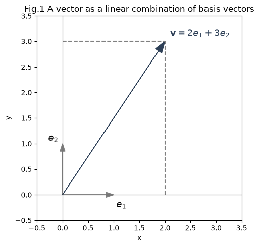

Inner products, norms, and orthogonality¶

The next natural operation multiplies two vectors into a number that measures how much they share a direction. Throughout this section, ${\color{orange} \vec a}$ is orange and ${\color{#3d81f6} \vec b}$ is blue, in every equation and every figure.

Definition: Dot product (computational form)

For ${\color{orange} \vec a}, {\color{#3d81f6} \vec b}$ with $n$ components, the dot product (in quantum notation, the inner product $\langle {\color{orange} a} \mid {\color{#3d81f6} b} \rangle$ ) is the scalar

{\color{orange} \vec a} \cdot {\color{#3d81f6} \vec b} = {\color{orange} \begin{pmatrix} a_1 \\ a_2 \\ \vdots \\ a_n \end{pmatrix}} \cdot {\color{#3d81f6} \begin{pmatrix} b_1 \\ b_2 \\ \vdots \\ b_n \end{pmatrix}} = {\color{orange} a_1}{\color{#3d81f6} b_1} + {\color{orange} a_2}{\color{#3d81f6} b_2} + \cdots + {\color{orange} a_n}{\color{#3d81f6} b_n}.

(2)

A worked example, with every number wearing its vector’s color. For ${\color{orange} \vec a = \begin{pmatrix} 6 \\ 2 \end{pmatrix}}$ and ${\color{#3d81f6} \vec b = \begin{pmatrix} 5 \\ -3 \end{pmatrix}}$ :

{\color{orange} \vec a} \cdot {\color{#3d81f6} \vec b} = ({\color{orange} 6})({\color{#3d81f6} 5}) + ({\color{orange} 2})({\color{#3d81f6} -3}) = 30 - 6 = 24.

(3)

The two forms together are a machine for extracting angles from components. And the special case $\cos\theta = 0$ earns its own name:

Vectors that are both orthogonal and normalized are orthonormal, compactly written with the Kronecker delta:

\langle e_i \mid e_j \rangle = \delta_{ij} = \begin{cases} 1 & i = j \\ 0 & i \neq j \end{cases}.

(5)

The norm is the square root of a vector’s inner product with itself, giving its length:

\langle a \mid a \rangle = a_1^2 + a_2^2, \qquad \|a\| = \sqrt{a_1^2 + a_2^2}.

(6)

A vector with $\|a\| = 1$ is normalized.

Projection: the most quantum operation in this appendix¶

The answer defines the orthogonal projection. Choose $k$ so that the leftover error vector ${\color{#d81b60} \vec e} = {\color{orange} \vec a} - k{\color{#3d81f6} \vec b}$ is orthogonal to ${\color{#3d81f6} \vec b}$ ; any other choice leaves a longer error (Pythagoras). That choice gives:

a_v = np.array([2.0, 3.0])
b_v = np.array([4.0, 1.0])
p_v = (a_v @ b_v) / (b_v @ b_v) * b_v

fig_pr, ax_pr = plt.subplots(figsize=(6.4, 4.6))
s = np.linspace(-0.5, 1.35, 2)
ax_pr.plot(s * b_v[0], s * b_v[1], color="0.85", lw=1.2, zorder=0)
for vec, color, label, dx, dy in [
    (a_v, "orange", r"$\vec a$", -0.25, 0.15),
    (b_v, "#3d81f6", r"$\vec b$", 0.1, -0.3),
    (p_v, "#004d40", r"$\vec p$", 0.05, 0.22),
]:
    ax_pr.annotate("", xy=vec, xytext=(0, 0),
                   arrowprops=dict(arrowstyle="->", color=color, lw=2.6))
    ax_pr.text(vec[0] + dx, vec[1] + dy, label, color=color, fontsize=14)
ax_pr.plot([p_v[0], a_v[0]], [p_v[1], a_v[1]], "--", color="#d81b60", lw=2.2)
ax_pr.text((p_v[0] + a_v[0]) / 2 + 0.12, (p_v[1] + a_v[1]) / 2, r"$\vec e$",
           color="#d81b60", fontsize=14)
u_hat = b_v / np.linalg.norm(b_v)
n_hat = np.array([-u_hat[1], u_hat[0]])
sq = 0.16
corner = p_v
ax_pr.plot([corner[0] - sq * u_hat[0], corner[0] - sq * u_hat[0] + sq * n_hat[0]],
           [corner[1] - sq * u_hat[1], corner[1] - sq * u_hat[1] + sq * n_hat[1]],
           color="0.4", lw=1)
ax_pr.plot([corner[0] - sq * u_hat[0] + sq * n_hat[0], corner[0] + sq * n_hat[0]],
           [corner[1] - sq * u_hat[1] + sq * n_hat[1], corner[1] + sq * n_hat[1]],
           color="0.4", lw=1)
ax_pr.set_xlim(-0.8, 5.2)
ax_pr.set_ylim(-0.8, 3.6)
ax_pr.set_aspect("equal")
ax_pr.grid(True, ls=":", alpha=0.5)
ax_pr.set_title("the projection p is the shadow of a along b; the error e is orthogonal", fontsize=10)
plt.show()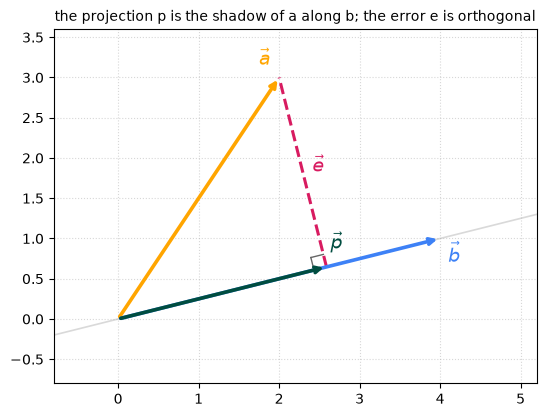

The picture contains a decomposition. Walking along ${\color{#004d40} \vec p}$ and then along ${\color{#d81b60} \vec e}$ lands exactly on ${\color{orange} \vec a}$ :

{\color{orange} \vec a} = \underbrace{{\color{#004d40} \vec p}}_{\text{parallel to } {\color{#3d81f6} \vec b}} + \underbrace{{\color{#d81b60} \vec e}}_{\text{orthogonal to } {\color{#3d81f6} \vec b}}.

(8)

Now the quantum payoff. For an orthonormal basis $\{e_1, e_2, \ldots\}$ the projection formula collapses to $c_k = \langle e_k \mid a \rangle$ , and expanding a vector in a basis is nothing but projecting it onto each basis direction in turn:

\vec a = \sum_k c_k\, e_k, \qquad c_k = \langle e_k \mid a \rangle.

(9)

In quantum mechanics the state $\psi$ is the vector, the eigenstates of a measurement are the orthonormal basis, and the numbers $|c_k|^2 = |\langle e_k \mid \psi \rangle|^2$ become the probabilities of each outcome (the Born rule). Every quantum measurement is, at its mathematical heart, the orthogonal projection drawn above.

Solution

$\langle v | v \rangle = 1^* \cdot 1 + i^* \cdot i = 1 + (-i)(i) = 1 + 1 = 2$ , so $\|\vec v\| = \sqrt{2}$ and the normalized vector is $\tfrac{1}{\sqrt 2}(1, i)$ . Forgetting the complex conjugate gives $1 + i^2 = 0$ : a nonzero vector with zero length, which is the classic sign you dropped the star.

Matrices¶

Linear systems as matrix equations¶

A system of linear equations is a matrix acting on a vector. The system

\begin{aligned} a_{11}x_1 + a_{12}x_2 &= b_1 \\ a_{21}x_1 + a_{22}x_2 &= b_2 \end{aligned}

(10)

packs into a single matrix-vector product:

Matrix times vector is the dot product of each row of $A$ with $\mathbf{x}$ :

A\mathbf{x} = \begin{pmatrix} a_{11}x_1 + a_{12}x_2 \\ a_{21}x_1 + a_{22}x_2 \end{pmatrix}.

(12)

If $A$ is invertible, the solution is $\mathbf{x} = A^{-1}\mathbf{b}$ .

import numpy as np

A = np.array([[2, 3],
              [1, -2]])
b = np.array([7, 1])

# Solve by inversion, and with the recommended solver
x_inv = np.linalg.inv(A) @ b
x_solve = np.linalg.solve(A, b)

print("solution via inverse:", x_inv)
print("solution via solve  :", x_solve)

solution via inverse: [2.42857143 0.71428571]
solution via solve  : [2.42857143 0.71428571]

Prefer solve over inv

np.linalg.solve(A, b) is both faster and more numerically accurate than forming np.linalg.inv(A) @ b. Inverting a matrix explicitly is almost never necessary and should be avoided in real calculations; we show the inverse here only because it makes the algebra transparent.

Eigenvalues and eigenvectors¶

When a matrix acts on a vector it usually changes both its length and direction. Certain special vectors keep their direction and are only rescaled. These are eigenvectors, and the scaling factors are eigenvalues.

Rearranging to $(A - \lambda I)\mathbf{v} = 0$ , a nonzero solution exists only when the characteristic equation holds:

\det(A - \lambda I) = 0.

(14)

The sign and size of $\lambda$ say what happens to the eigenvector: $\lambda > 1$ stretches it, $0 < \lambda < 1$ compresses it, $\lambda < 0$ flips it, and $\lambda = 0$ collapses it. In quantum mechanics this exact structure reappears for operators acting on wavefunctions: eigenvalues are the measurable observables (energies, momenta) and eigenvectors are the states with definite outcomes. The next page makes that leap explicit, showing that a function is just a vector with infinitely many components and the Schrodinger equation $\hat H\psi = E\psi$ is this same eigenvalue problem $A\mathbf{v}=\lambda\mathbf{v}$ .

import numpy as np

A = np.array([[2, 1],
              [1, 2]])
vals, vecs = np.linalg.eig(A)

print("eigenvalues :", vals)
print("eigenvectors (columns):\n", vecs)

# Verify A v = lambda v for the first eigenpair
print("\nA @ v0        :", A @ vecs[:, 0])
print("lambda0 * v0  :", vals[0] * vecs[:, 0])

eigenvalues : [3.+0.j 1.+0.j]
eigenvectors (columns):
 [[ 0.70710678+0.j -0.70710678+0.j]
 [ 0.70710678+0.j  0.70710678+0.j]]

A @ v0        : [2.12132034+0.j 2.12132034+0.j]
lambda0 * v0  : [2.12132034+0.j 2.12132034+0.j]

The whole story in one picture: a matrix turns almost every vector, but an eigenvector comes back parallel to itself.

A_eig = np.array([[2, 1], [1, 2]])
w = np.array([1.0, -0.35])
u = np.array([1.0, 1.0]) / np.sqrt(2)

fig_e, (axg, axe) = plt.subplots(1, 2, figsize=(9, 4.4))
for ax_, v1, v2, c1, c2, ttl in [
    (axg, w, A_eig @ w, "0.45", "steelblue", "a generic vector turns"),
    (axe, u, A_eig @ u, "0.45", "crimson", "an eigenvector only stretches"),
]:
    ax_.annotate("", xy=v1, xytext=(0, 0), arrowprops=dict(arrowstyle="->", color=c1, lw=2.5))
    ax_.annotate("", xy=v2, xytext=(0, 0), arrowprops=dict(arrowstyle="->", color=c2, lw=2.5))
    ax_.text(*(v1 * 1.15), r"$\vec{v}$", color=c1, fontsize=13)
    ax_.text(*(v2 * 1.06), r"$A\vec{v}$", color=c2, fontsize=13)
    ax_.set_xlim(-0.6, 3.0); ax_.set_ylim(-1.2, 2.6)
    ax_.set_aspect("equal"); ax_.grid(True, ls=":", alpha=0.6)
    ax_.set_title(ttl, fontsize=11)
fig_e.tight_layout()
plt.show()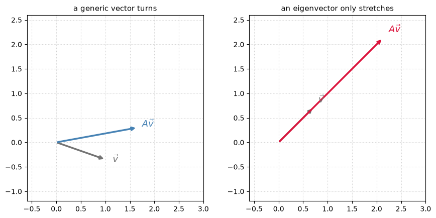

On the left, $\vec v$ (gray) and $\color{steelblue} A\vec v$ (blue) point in different directions: the matrix rotated the vector. On the right, the eigenvector $\vec u = \tfrac{1}{\sqrt 2}(1,1)$ obeys $\color{crimson} A\vec u = 3\vec u$ : same direction, three times longer. Eigenvectors are the directions along which a matrix acts like simple multiplication.

Solution

$\det(\sigma_x - \lambda I) = \lambda^2 - 1 = 0$ gives $\lambda = \pm 1$ : the two possible outcomes of the measurement. For $\lambda = +1$ : $\vec v_+ = \tfrac{1}{\sqrt 2}(1, 1)$ ; for $\lambda = -1$ : $\vec v_- = \tfrac{1}{\sqrt 2}(1, -1)$ . These are exactly the spin-right and spin-left states of Chapter 5, and note they are orthogonal, as eigenvectors of distinct eigenvalues of a symmetric matrix must be.

The geometric action of a matrix¶

Different kinds of matrices deform a shape in characteristic ways:

Matrix type	Example	Effect
Diagonal, unequal entries	`[[1.8, 0], [0, 0.8]]`	Stretch, different scaling per axis
Diagonal, equal entries	`[[0.7, 0], [0, 0.7]]`	Uniform scaling
Rotation (orthogonal)	`[[cosθ, -sinθ], [sinθ, cosθ]]`	Rotation, preserves lengths and angles
Off-diagonal term	`[[1, k], [0, 1]]`	Shear, slants without changing area

We apply each matrix to the same small polygon to see how it transforms.

import numpy as np
import matplotlib.pyplot as plt

coords = np.array([[0, 0], [0.5, 0.5], [0.5, 1.5], [0, 1], [0, 0]]).T

stretch = np.array([[1.8, 0], [0, 0.8]])
rotation = np.array([[np.cos(np.pi / 6), -np.sin(np.pi / 6)],
                     [np.sin(np.pi / 6),  np.cos(np.pi / 6)]])
shear = np.array([[1, 0.8], [0, 1]])
scaling = np.array([[0.7, 0], [0, 0.7]])

transforms = {
    "Stretch (non-uniform)": stretch,
    "Rotation (30 deg)": rotation,
    "Shear": shear,
    "Scaling (uniform)": scaling,
}

fig, axes = plt.subplots(2, 2, figsize=(8, 8))
for ax, (name, M) in zip(axes.flat, transforms.items()):
    ax.plot(coords[0], coords[1], 'r--', label='original')
    new_coords = M @ coords
    ax.plot(new_coords[0], new_coords[1], 'b-', label='transformed')
    ax.set_title(name, fontsize=11)
    ax.set_aspect('equal', 'box')
    ax.set_xlim(-2, 2)
    ax.set_ylim(-1, 2)
    ax.grid(True, ls=':')
    ax.legend(fontsize=8, loc='upper left')

plt.suptitle('Fig.2 How different matrices deform the same shape', fontsize=13)
plt.tight_layout()
plt.show()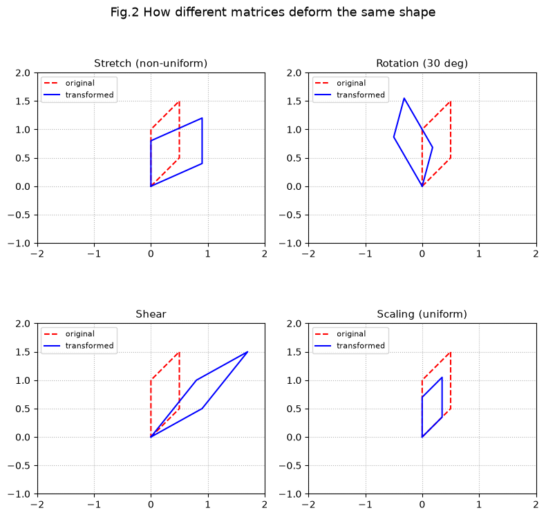

A matrix in new axes: diagonalization¶

Turning the axes changes the components of a vector but not the vector, as in the tip on bases at the start of this page. A matrix is the same: its entries depend on the axes, while what it does to an arrow does not.

In the usual axes $\mathbf{e}_1 = (1, 0)$ and $\mathbf{e}_2 = (0, 1)$ , the entry in row $m$ and column $n$ is a dot product, $A_{mn} = \mathbf{e}_m \cdot (A\mathbf{e}_n)$ : the matrix turns $\mathbf{e}_n$ into $A\mathbf{e}_n$ , and the entry says how much of that lands on $\mathbf{e}_m$ . Turn to any two perpendicular unit vectors $\mathbf{u}_1$ and $\mathbf{u}_2$ and the same recipe gives the matrix in the new axes. In Dirac’s notation it is a “sandwich” of a bra, the matrix and a ket:

A'_{mn} = \mathbf{u}_m \cdot (A\mathbf{u}_n) = \langle \mathbf{u}_m \mid A \mid \mathbf{u}_n \rangle

(15)

The matrix has not changed: it turns and stretches every arrow exactly as before. Only its description changes.
Read column $n$ of $A'$ as the arrow $A\mathbf{u}_n$ written in the new axes. The diagonal entry $A'_{nn}$ is the part of $A\mathbf{u}_n$ along its own axis; the off-diagonal entry is the part that lands on the other axis.

Try it: drag on the plane to turn the axes for $A = \begin{pmatrix} 2 & 1 \\ 1 & 2 \end{pmatrix}$ , the matrix of the eigenvalue picture above. The orange pieces are the off-diagonal entries. They shrink as you turn, and at $45^\circ$ they vanish: each $A\mathbf{u}_n$ then lies along its own axis. The trace and the determinant never change.

For this $A$ , axes turned by an angle $\theta$ , with $\mathbf{u}_1 = (\cos\theta, \sin\theta)$ and $\mathbf{u}_2 = (-\sin\theta, \cos\theta)$ , give

A'(\theta) = \begin{pmatrix} 2 + \sin 2\theta & \cos 2\theta \\ \cos 2\theta & 2 - \sin 2\theta \end{pmatrix}

(16)

The off-diagonal entry $\cos 2\theta$ vanishes at $\theta = 45^\circ$ . The trace is 4 and the determinant is $4 - \sin^2 2\theta - \cos^2 2\theta = 3$ at every angle, so the eigenvalues, the roots of $\lambda^2 - 4\lambda + 3 = 0$ , cannot change when the axes turn.

Example: diagonal in its own eigenbasis

Write $A = \begin{pmatrix} 2 & 1 \\ 1 & 2 \end{pmatrix}$ in the axes of its eigenvectors, $\mathbf{u}_1 = \tfrac{1}{\sqrt{2}}(1, 1)$ and $\mathbf{u}_2 = \tfrac{1}{\sqrt{2}}(1, -1)$ .

Each eigenvector is only stretched, $A\mathbf{u}_1 = 3\,\mathbf{u}_1$ and $A\mathbf{u}_2 = \mathbf{u}_2$ , so every sandwich is an eigenvalue times an overlap, $\langle \mathbf{u}_m \mid A \mid \mathbf{u}_n \rangle = \lambda_n \langle \mathbf{u}_m \mid \mathbf{u}_n \rangle$ . The axes are perpendicular unit vectors, so the overlap is 1 for $m = n$ and 0 otherwise:

A' = \begin{pmatrix} 3\cdot 1 & 1\cdot 0 \\ 3\cdot 0 & 1\cdot 1 \end{pmatrix} = \begin{pmatrix} 3 & 0 \\ 0 & 1 \end{pmatrix}

(17)

Check one entry by row times column: $A\mathbf{u}_1 = \tfrac{1}{\sqrt{2}}(3, 3)$ , so $\langle \mathbf{u}_2 \mid A \mid \mathbf{u}_1 \rangle = \tfrac{1}{2}\big(1\cdot 3 + (-1)\cdot 3\big) = 0$ . The trace is still $3 + 1 = 4$ and the determinant $3 \times 1 = 3$ .

Finding those axes is called diagonalizing the matrix. A symmetric matrix always has perpendicular unit eigenvectors (so does a Hermitian one, see Operators as Matrices), so it can always be diagonalized. In numpy, eigh returns the eigenvectors as the columns of a matrix U, and U.T @ A @ U computes every sandwich $\langle \mathbf{u}_m \mid A \mid \mathbf{u}_n \rangle$ at once: row $m$ of U.T is the bra, column $n$ of U the ket.

import numpy as np

A_ax = np.array([[2.0, 1.0], [1.0, 2.0]])
lam_ax, U_ax = np.linalg.eigh(A_ax)              # columns of U_ax: the eigenvectors, the new axes
A_ax_new = U_ax.T @ A_ax @ U_ax                  # every sandwich at once

print("eigenvalues        :", lam_ax)            # eigh lists them in increasing order
print("A in the new axes  :\n", np.round(A_ax_new, 10) + 0.0)    # adding 0.0 prints -0. as 0.
print("trace before, after:", np.trace(A_ax), round(np.trace(A_ax_new), 10))
print("det   before, after:", round(np.linalg.det(A_ax), 10), round(np.linalg.det(A_ax_new), 10))

eigenvalues        : [1. 3.]
A in the new axes  :
 [[1. 0.]
 [0. 3.]]
trace before, after: 4.0 4.0
det   before, after: 3.0 3.0

The new matrix is diagonal, with the eigenvalues 1 and 3 in increasing order, and the trace and determinant are unchanged. This is what “diagonalizing a Hamiltonian” means in Operators 1: find the eigenvectors of $H$ , write $H$ in those axes, and read the energies off the diagonal. For complex matrices the bra carries a complex conjugate, U.conj().T @ A @ U.

Problems¶

Problem 1: Dot product and angle¶

Find $\langle a \mid b \rangle$ and the angle between $a = (1, 2)$ and $b = (3, -1)$ .

Solution

\langle a \mid b \rangle = (1)(3) + (2)(-1) = 1.

(19)

With $|a| = \sqrt{5}$ and $|b| = \sqrt{10}$ ,

\cos\theta = \frac{1}{\sqrt{5}\sqrt{10}} = \frac{1}{\sqrt{50}} \approx 0.141, \qquad \theta \approx 81.9^\circ.

(20)

Problem 2: Normalize a vector¶

Normalize $v = (3, 4)$ .

Solution

$|v| = \sqrt{9 + 16} = 5$ , so the normalized vector is $\hat{v} = (3/5,\ 4/5)$ , which has length 1.

Problem 3: Check orthogonality¶

Are $(1, 1)$ and $(1, -1)$ orthogonal? Are they orthonormal?

Solution

Their dot product is $(1)(1) + (1)(-1) = 0$ , so they are orthogonal. Each has length $\sqrt{2}$ , not 1, so they are orthogonal but not orthonormal. Dividing each by $\sqrt{2}$ makes them orthonormal.

Problem 4: Eigenvalues by hand¶

Find the eigenvalues of $A = \begin{pmatrix} 2 & 1 \\ 1 & 2 \end{pmatrix}$ .

Solution

\det(A - \lambda I) = (2 - \lambda)^2 - 1 = 0 \;\Rightarrow\; (2-\lambda) = \pm 1,

(21)

so $\lambda = 3$ and $\lambda = 1$ , matching the numerical output above.

Problem 5: Solve a linear system¶

Solve $\begin{pmatrix} 2 & 3 \\ 1 & -2 \end{pmatrix}\mathbf{x} = \begin{pmatrix} 7 \\ 1 \end{pmatrix}$ by hand and check against the code.

Problem 6: Rotation preserves length¶

Show that the rotation matrix $R = \begin{pmatrix} \cos\theta & -\sin\theta \\ \sin\theta & \cos\theta \end{pmatrix}$ leaves the norm of any vector unchanged.

Problem 7: Eigenvector direction¶

Verify that $(1, 1)$ is an eigenvector of $A = \begin{pmatrix} 2 & 1 \\ 1 & 2 \end{pmatrix}$ and identify its eigenvalue.

Problem 8: Complex inner product¶

For complex vectors the inner product conjugates the first entry: $\langle a \mid b \rangle = \sum_i a_i^* b_i$ . Compute $\langle a \mid a \rangle$ for $a = (1,\ i)$ and confirm it is real and positive.