Div, Grad, Curl and All That - Quantum Mechanics for Chemistry

What you need to know

The operator $\nabla$ (“del”) is a vector of derivatives. Applied three different ways, it asks three different local questions about a field:
- Gradient $\nabla f$ : which way is uphill, and how steep? (scalar in, vector out)
- Divergence $\nabla \cdot \mathbf{F}$ : is this point a source or a sink? (vector in, scalar out)
- Curl $\nabla \times \mathbf{F}$ : does the field rotate around this point? (vector in, vector out)
Gradient and curl are not just bookkeeping: the gradient generates translations and the curl direction is tied to rotations. In quantum mechanics these become the momentum operator $\hat{p} = -i\hbar \nabla$ and the angular momentum operator $\hat{L} = -i\hbar\, \mathbf{r}\times\nabla$ .
The Laplacian $\nabla^2 = \nabla \cdot \nabla$ measures “how different I am from the average of my neighbors.” It drives diffusion, and it is the kinetic energy in the Schrödinger equation.
The title honors the classic little book by Schey Schey, 2005, which every chemist secretly keeps within reach.

The del operator¶

In Cartesian coordinates del is simply

\nabla = \left( \frac{\partial}{\partial x}, \; \frac{\partial}{\partial y}, \; \frac{\partial}{\partial z} \right),

(1)

a vector whose components are “slope detectors” along each axis. Everything on this page is one object applied three ways: multiply it onto a scalar ( $\nabla f$ ), dot it into a vector ( $\nabla \cdot \mathbf{F}$ ), or cross it into a vector ( $\nabla \times \mathbf{F}$ ).

1. Gradient: the uphill compass¶

For a scalar landscape $f(x, y)$ , the gradient $\nabla f$ at each point aims in the direction of steepest increase, with length equal to the slope. Contour lines are always crossed at right angles.

import numpy as np
import matplotlib.pyplot as plt

x = np.linspace(-2, 2, 300)
X, Y = np.meshgrid(x, x)
H = np.exp(-((X - 0.5)**2 + (Y - 0.3)**2)) + 0.7 * np.exp(-2*((X + 0.9)**2 + (Y + 0.7)**2))

xs = np.linspace(-2, 2, 18)
Xq, Yq = np.meshgrid(xs, xs)
Hq = np.exp(-((Xq - 0.5)**2 + (Yq - 0.3)**2)) + 0.7 * np.exp(-2*((Xq + 0.9)**2 + (Yq + 0.7)**2))
dHy, dHx = np.gradient(Hq, xs, xs)

fig, ax = plt.subplots(figsize=(6.5, 5.2))
cs = ax.contourf(X, Y, H, levels=18, cmap="terrain")
ax.contour(X, Y, H, levels=18, colors="k", linewidths=0.3, alpha=0.4)
ax.quiver(Xq, Yq, dHx, dHy, color="crimson", width=0.004, scale=12)
ax.set_aspect("equal")
ax.set_title("gradient arrows point uphill, perpendicular to contours", fontsize=11)
ax.set_xlabel("x"); ax.set_ylabel("y")
fig.colorbar(cs, ax=ax, shrink=0.85, label="height f(x, y)")
fig.tight_layout()
plt.show()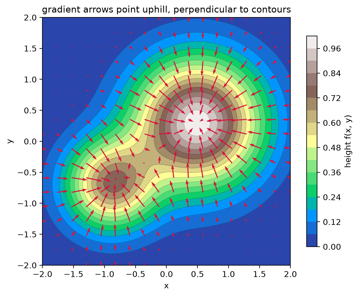

Two physical readings, both constant companions in this course:

Diffusion runs downhill. Fick’s law says the flux of concentration is $\mathbf{J} = -D \nabla c$ : matter flows from crowded regions to empty ones, exactly opposite to the gradient. The same minus sign makes forces run downhill in energy, $\mathbf{F} = -\nabla V$ .
The gradient generates translation, and this deserves its own moment.

The derivative is a translation machine¶

Write out Taylor’s theorem for a shift by $a$ and stare at its structure:

f(x + a) \;=\; f(x) + a\,\frac{df}{dx} + \frac{a^2}{2!}\,\frac{d^2 f}{dx^2} + \frac{a^3}{3!}\,\frac{d^3 f}{dx^3} + \cdots \;=\; \sum_{n=0}^{\infty} \frac{1}{n!}\left(a \frac{d}{dx}\right)^{\! n} f(x).

(2)

The right-hand side is exactly the exponential series, applied to an operator instead of a number:

f(x + a) = e^{\,a\, d/dx} \, f(x).

(3)

Exponentiating the derivative slides a function sideways. The figure below makes this concrete: keep more and more terms of the operator series and watch a Gaussian being carried to its translated position, term by term.

xg = np.linspace(-4, 6, 1024)
f0 = np.exp(-xg**2)
a_shift = 2.0

k = 2 * np.pi * np.fft.fftfreq(len(xg), xg[1] - xg[0])
F0 = np.fft.fft(f0)

fig6, ax6 = plt.subplots(figsize=(7.5, 4))
ax6.plot(xg, f0, lw=2, color="0.55", label="f(x)")
colors = plt.cm.plasma(np.linspace(0.15, 0.8, 4))
for Nmax, c in zip([1, 2, 4, 12], colors):
    op = np.zeros_like(F0)
    term = np.ones_like(F0)
    for n_t in range(Nmax + 1):
        op = op + term
        term = term * (1j * k * a_shift) / (n_t + 1)
    fN = np.fft.ifft(F0 * op).real
    ax6.plot(xg, fN, lw=1.7, color=c, label=f"series through n = {Nmax}")
ax6.plot(xg, np.exp(-(xg - a_shift)**2), "k--", lw=2, label="exact f(x - (-a)) target")
ax6.set_ylim(-0.4, 1.35)
ax6.set_xlabel("x")
ax6.set_title(r"partial sums of $e^{a\,d/dx}$ carry the function to its shifted self", fontsize=11)
ax6.legend(fontsize=8, frameon=False, ncol=2)
fig6.tight_layout()
plt.show()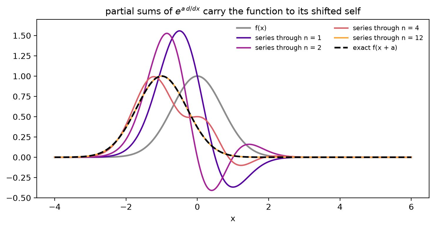

One term tilts the function, two terms lean it further, and by a dozen terms the series has physically moved it. Now the quantum punchline: multiply the generator by $-i\hbar$ and you get the momentum operator $\hat{p} = -i\hbar\, d/dx$ , so that

e^{\,i a \hat{p} / \hbar}\, \psi(x) = \psi(x + a).

(4)

This is where momentum comes from. Momentum is not defined by $mv$ in quantum mechanics; it is defined as the generator of translations, the operator whose exponential slides wavefunctions through space. That a particle in empty space conserves momentum is then just the statement that empty space looks the same after any slide (Noether’s theorem in one sentence).

2. Divergence: sources and sinks¶

Dot del into a vector field and you get a number at each point:

\nabla \cdot \mathbf{F} = \frac{\partial F_x}{\partial x} + \frac{\partial F_y}{\partial y} + \frac{\partial F_z}{\partial z}.

(5)

The number answers: does more field leave this point than enters it? Positive divergence marks a source (a faucet), negative marks a sink (a drain). Equivalently, if the field were a fluid velocity, $\nabla \cdot \mathbf{v}$ is the fractional rate at which a small blob of fluid expands: divergence measures outward translation of volume.

xs2 = np.linspace(-2.5, 2.5, 24)
X2, Y2 = np.meshgrid(xs2, xs2)
R2 = X2**2 + Y2**2
Fx = X2 * np.exp(-R2 / 2)
Fy = Y2 * np.exp(-R2 / 2)
div = np.gradient(Fx, xs2, axis=1) + np.gradient(Fy, xs2, axis=0)

fig2, ax2 = plt.subplots(figsize=(6.2, 5.2))
pc = ax2.pcolormesh(X2, Y2, div, cmap="RdBu_r", shading="gouraud",
                    vmin=-np.abs(div).max(), vmax=np.abs(div).max())
ax2.quiver(X2, Y2, Fx, Fy, width=0.004, scale=14)
ax2.set_aspect("equal")
ax2.set_title("a source field: red = positive divergence (faucet), blue = negative (drain)", fontsize=10)
ax2.set_xlabel("x"); ax2.set_ylabel("y")
fig2.colorbar(pc, ax=ax2, shrink=0.85, label=r"$\nabla \cdot \mathbf{F}$")
fig2.tight_layout()
plt.show()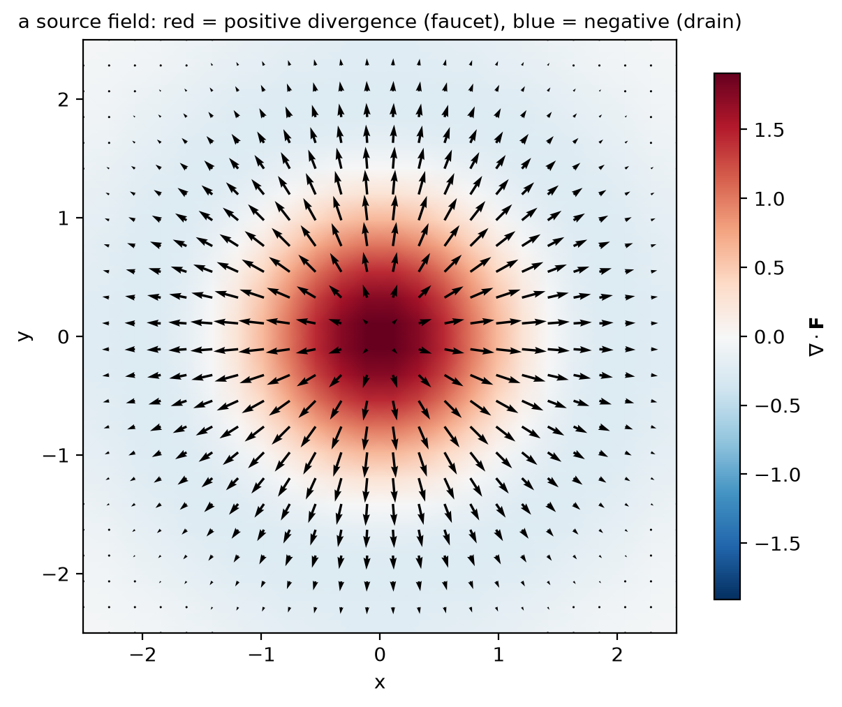

The field above gushes out of the origin (red center) and, because the arrows fade with distance, the far region acts as a gentle drain (blue ring). Electrostatics is exactly this picture: Gauss’s law $\nabla \cdot \mathbf{E} = \rho / \varepsilon_0$ says electric charge is the faucet of the electric field. Where there is no charge, field lines just pass through.

3. Curl: the paddle wheel¶

Cross del into a vector field and you get a vector whose direction is the local axis of rotation and whose magnitude is twice the local spin rate. The classic test: drop a tiny paddle wheel into the flow; if it turns, the curl is nonzero, and it points along the wheel’s axle by the right-hand rule.

Gx = -Y2 * np.exp(-R2 / 2)
Gy = X2 * np.exp(-R2 / 2)
curl_z = np.gradient(Gy, xs2, axis=1) - np.gradient(Gx, xs2, axis=0)

fig3, ax3 = plt.subplots(figsize=(6.2, 5.2))
pc3 = ax3.pcolormesh(X2, Y2, curl_z, cmap="PuOr_r", shading="gouraud",
                     vmin=-np.abs(curl_z).max(), vmax=np.abs(curl_z).max())
ax3.quiver(X2, Y2, Gx, Gy, width=0.004, scale=14)
ax3.set_aspect("equal")
ax3.set_title("a vortex: the paddle wheel spins fastest in the orange core", fontsize=11)
ax3.set_xlabel("x"); ax3.set_ylabel("y")
fig3.colorbar(pc3, ax=ax3, shrink=0.85, label=r"$(\nabla \times \mathbf{F})_z$")
fig3.tight_layout()
plt.show()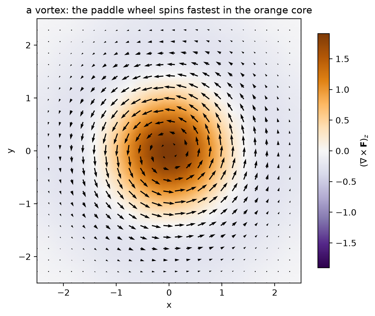

This is a vortex: the same field a stirred cup of coffee has, and fluid dynamicists call $\boldsymbol{\omega} = \nabla \times \mathbf{v}$ the vorticity. Rotation is the curl’s whole personality, and that connection survives into quantum mechanics: the operator that generates rotations is the angular momentum $\hat{L} = -i\hbar \, \mathbf{r} \times \nabla$ , built from position crossed with the gradient exactly the way curl crosses del into a field.

Magnetostatics is the curl picture: Ampère’s law $\nabla \times \mathbf{B} = \mu_0 \mathbf{J}$ says electric currents stir the magnetic field into closed loops around them.

Electric vs magnetic: a tale of two operators¶

Nature staged the perfect comparison experiment. A point charge builds a field that is all divergence and no curl; a straight current builds one that is all curl and no divergence. Same del, opposite personalities:

xs4 = np.linspace(-2, 2, 200)
X4, Y4 = np.meshgrid(xs4, xs4)
R4 = np.sqrt(X4**2 + Y4**2) + 1e-9

Ex, Ey = X4 / R4**2, Y4 / R4**2          # point charge (2D)
Bx, By = -Y4 / R4**2, X4 / R4**2         # wire along z

fig4, (axE, axB) = plt.subplots(1, 2, figsize=(10, 4.6))
for ax_, (Ux, Uy), title in [
    (axE, (Ex, Ey), "electric field of a charge: all divergence, zero curl"),
    (axB, (Bx, By), "magnetic field of a wire: all curl, zero divergence"),
]:
    speed = np.hypot(Ux, Uy)
    ax_.streamplot(X4, Y4, Ux, Uy, color=np.log(speed), cmap="viridis",
                   density=1.1, linewidth=1, arrowsize=1.2)
    ax_.plot(0, 0, "o", ms=10, color="crimson")
    ax_.set_aspect("equal")
    ax_.set_title(title, fontsize=10)
    ax_.set_xlim(-2, 2); ax_.set_ylim(-2, 2)
axE.set_ylabel("y")
axE.set_xlabel("x"); axB.set_xlabel("x")
fig4.tight_layout()
plt.show()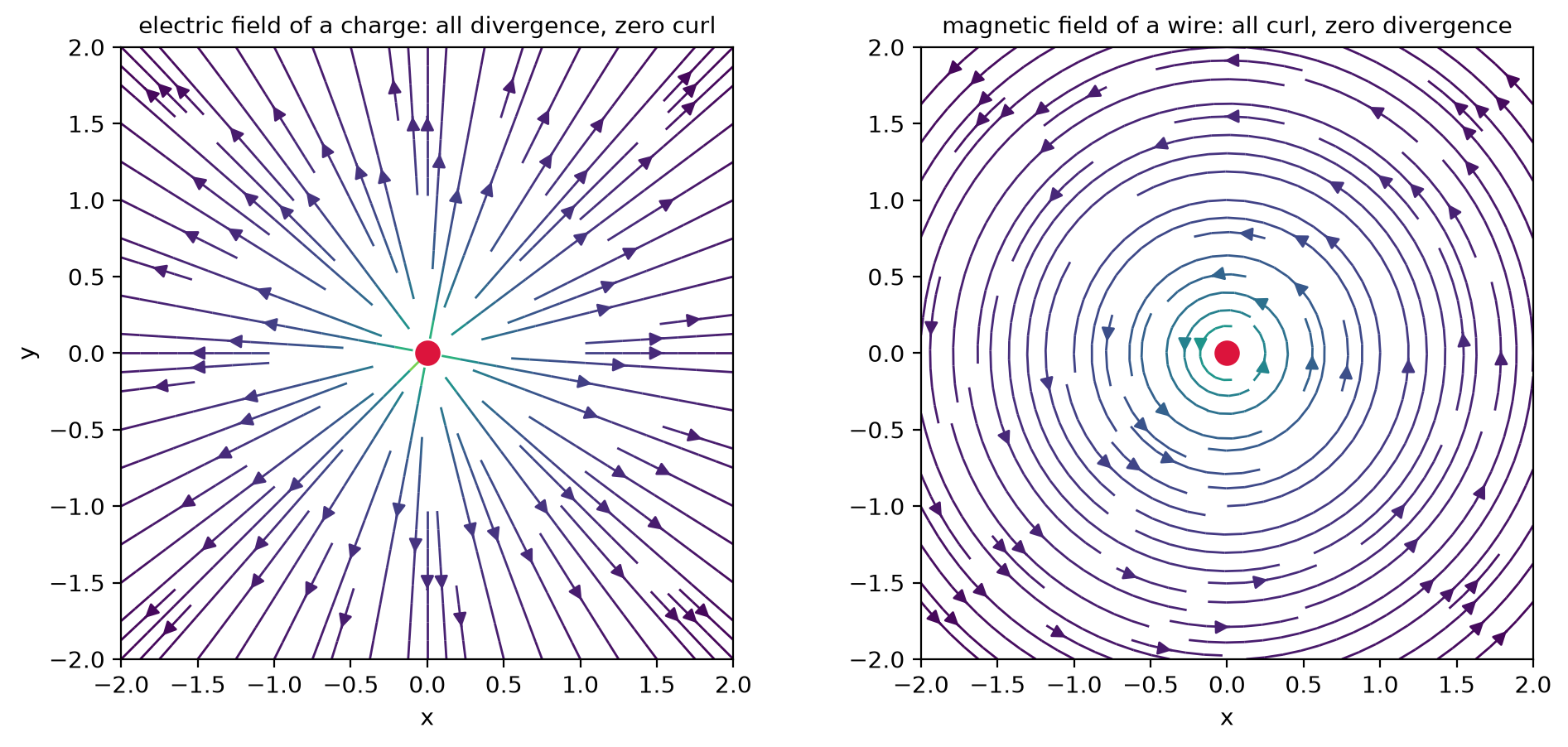

The absence of magnetic divergence, $\nabla \cdot \mathbf{B} = 0$ everywhere, is one of Maxwell’s equations and a factual statement about our universe: nobody has ever found a magnetic faucet (a monopole). Field lines of $\mathbf{B}$ have no choice but to close on themselves.

Mix your own field¶

Every smooth field can be split into a curl-free part and a divergence-free part (the Helmholtz decomposition), so the two examples above are the primary colors of vector calculus. Blend them yourself: the slider rotates a field from pure source to pure vortex, and the labels report the divergence and curl it carries.

Watch the trade: as the angle grows, divergence drains out of the field and reappears as curl. At 45 degrees the field spirals, half faucet and half whirlpool, the way a draining bathtub combines both.

The Laplacian: how diffusion thinks¶

Apply del twice, $\nabla^2 f = \nabla \cdot (\nabla f)$ , and you get the Laplacian: a number that compares $f$ at a point with the average of its immediate neighbors. Positive $\nabla^2 f$ means “my neighbors are higher than me” (a dimple), negative means “I stick out” (a bump).

The cleanest way to see this is the discrete stencil from numerical calculus:

\nabla^2 f \Big|_{x} \;\approx\; \frac{f(x+h) + f(x-h) - 2 f(x)}{h^2} \;=\; \frac{2}{h^2} \Big( \underbrace{\tfrac{f(x+h) + f(x-h)}{2}}_{\text{neighbor average}} - \; f(x) \Big).

(6)

The Laplacian is “neighbor average minus me,” rescaled. The figure below shows a lumpy concentration profile, its neighbor average, and the resulting push: wherever the curve sits above its neighbors’ average the Laplacian is negative and diffusion pushes it down; wherever it dips below, diffusion pushes it up.

xl = np.linspace(0, 10, 400)
prof = (1.1 * np.exp(-(xl - 2.4)**2 / 0.35) + 0.8 * np.exp(-(xl - 5.4)**2 / 1.8)
        - 0.45 * np.exp(-(xl - 8.0)**2 / 0.5) + 0.9)
lap = np.gradient(np.gradient(prof, xl), xl)

fig7, ax7 = plt.subplots(figsize=(7.5, 4))
ax7.plot(xl, prof, lw=2.4, color="steelblue", label="concentration c(x)")
sm = np.convolve(prof, np.ones(25) / 25, mode="same")
ax7.plot(xl[15:-15], sm[15:-15], lw=1.6, ls="--", color="0.45", label="neighbor average")
step = 16
for xi, ci, li in zip(xl[::step], prof[::step], lap[::step]):
    ax7.annotate("", xy=(xi, ci + np.clip(li, -0.9, 0.9) * 0.35), xytext=(xi, ci),
                 arrowprops=dict(arrowstyle="->", color="crimson", lw=1.4))
ax7.set_xlabel("x")
ax7.set_ylabel("c(x)")
ax7.set_title("red arrows: the push of the Laplacian, toward the neighbor average", fontsize=11)
ax7.legend(fontsize=9, frameon=False)
fig7.tight_layout()
plt.show()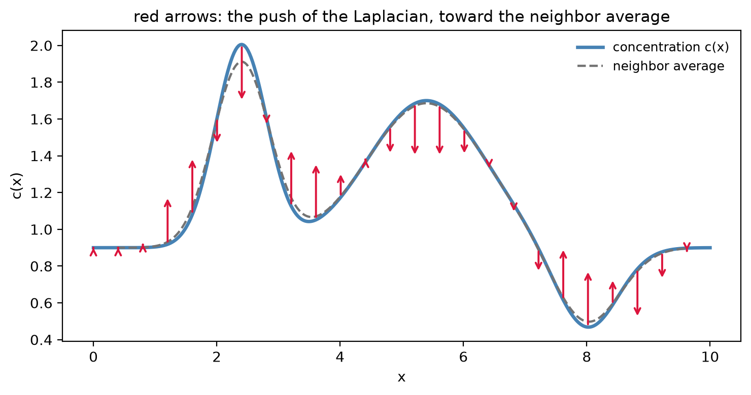

That push is precisely what diffusion obeys. The diffusion equation $\partial c / \partial t = D \nabla^2 c$ says: bumps melt, dimples fill, each point relaxing toward the average of its neighbors until nothing has anything to complain about (equilibrium).

xd = np.linspace(-6, 6, 400)
fig5, ax5 = plt.subplots(figsize=(7, 4))
for tt, color in [(0.15, "crimson"), (0.6, "darkorange"), (2.0, "steelblue"), (6.0, "seagreen")]:
    c = np.exp(-xd**2 / (4 * tt)) / np.sqrt(4 * np.pi * tt)
    ax5.plot(xd, c, lw=2.2, color=color, label=f"t = {tt}")
ax5.set_xlabel("x"); ax5.set_ylabel("concentration c(x, t)")
ax5.set_title("diffusion in action: the Laplacian melts the peak and fills the wings", fontsize=11)
ax5.legend(frameon=False)
fig5.tight_layout()
plt.show()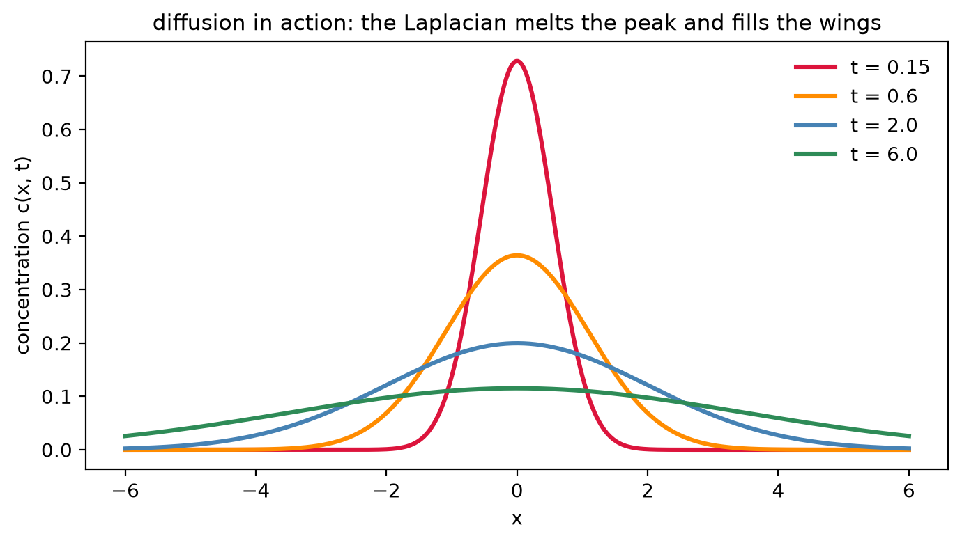

And now the payoff for this course: the Schrödinger equation’s kinetic energy is $-\frac{\hbar^2}{2m}\nabla^2$ . The same operator that makes ink spread through water measures how sharply a wavefunction bends, and sharp bending costs kinetic energy. When Chapter 3 tells you that squeezing a particle raises its energy, it is the Laplacian doing the telling.

The whole family at a glance¶

Operator	Input to output	Local question	Physics it runs	Quantum appearance
$\nabla f$	scalar to vector	which way is uphill?	Fick’s law, forces $\mathbf{F} = -\nabla V$	momentum $\hat{p} = -i\hbar\nabla$ generates translation
$\nabla \cdot \mathbf{F}$	vector to scalar	source or sink?	Gauss’s law $\nabla \cdot \mathbf{E} = \rho/\varepsilon_0$	probability conservation (continuity equation)
$\nabla \times \mathbf{F}$	vector to vector	does it rotate?	Ampère’s law, vorticity	$\hat{L} = -i\hbar\,\mathbf{r}\times\nabla$ generates rotation
$\nabla^2 f$	scalar to scalar	do I differ from my neighbors?	diffusion $\partial_t c = D\nabla^2 c$	kinetic energy $-\tfrac{\hbar^2}{2m}\nabla^2$

References¶

Schey, H. M. (2005). Div, Grad, Curl, and All That: An Informal Text on Vector Calculus (4th ed.). W. W. Norton.