Calculus Essentials - Quantum Mechanics for Chemistry

What you will learn

The derivative as a slope and as a step. The derivative is the slope of the tangent line, and read the other way it is the recipe for stepping from $f(x)$ to a neighboring value $f(x+h)$ .
Reading first and second derivatives. The sign of $f'$ says whether $f$ rises or falls, and $f''$ says how the curve bends. Together they locate and classify maxima, minima, and inflection points; in mechanics they are velocity and acceleration.
Taylor series. Each further derivative at a point predicts the function farther away; the full series reconstructs it exactly.
The rules of differentiation. Constant multiple, sum, product, quotient, power, and chain rules let you differentiate almost any function you meet in chemistry.
The integral as accumulated area. A definite integral is the limit of a sum of thin rectangles, giving the net area under a curve.
The fundamental theorem of calculus. Differentiation and integration are inverse operations, and this theorem is the workhorse for evaluating integrals.
Partial derivatives. When a function depends on several variables, differentiate with respect to one while holding the others fixed. The chain rule then shows that any shape sliding at constant speed, $f(x - vt)$ , obeys a simple relation between its space and time derivatives.
Techniques of integration. Substitution, integration by parts, and trigonometric identities handle almost every integral in this course.

Calculus is the language of change. Chemistry is full of quantities that vary with position, time, temperature, or pressure, and two questions come up again and again: how fast does a quantity change, which is a derivative, and how much of it accumulates, which is an integral. Later in the course the same two operations act on the functions that describe waves and, eventually, quantum states, so it pays to have them at your fingertips now. This page collects the essentials with a picture for each of the two ideas that matter most: the derivative as a slope and the integral as an area. In between sits a short section on partial derivatives, the small extension needed when a function depends on more than one variable, such as a wave $u(x,t)$ that depends on both position and time.

Differentiation¶

The derivative as a slope¶

The derivative of $f$ at a point is the slope of the line tangent to the curve there. We build it from the slope of a secant line through two nearby points and then let those points merge:

As the spacing $h$ shrinks, the secant line pivots into the tangent line. Drag the slider below for $f(x) = x^2$ at $x = 1$ : the secant slope $2 + h$ closes in on the true tangent slope 2.

The derivative is also the instantaneous rate of change: if $f$ is position, $f'$ is velocity; if $f$ is concentration, $f'$ is reaction rate. A function is differentiable only where it is smooth, so no corners, jumps, or vertical tangents.

The derivative as a step¶

Read the definition backwards and it becomes a recipe for moving along the curve. For a small step $h$ ,

f(x + h) \approx f(x) + f'(x)\,h .

(2)

Knowing the value and the slope at one position is enough to predict the value at a neighboring position: the derivative is the rate at which $f$ responds to a shift in $x$ . The green bar in the slider figure measures how far this prediction misses the true $f(x+h)$ . For $x^2$ the miss is exactly $h^2$ , so halving the step quarters the error, and in the limit the prediction is perfect. That is what “linear approximation” means, and it is why a tangent line is the best straight-line stand-in for a curve near a point.

Higher derivatives predict farther: the Taylor series¶

The step recipe uses one derivative and works for small steps. Each further derivative extends the reach, and with all of them the prediction becomes exact for any smooth function:

The first two terms are the step recipe (the linear approximation). Adding the $a^2$ term corrects for the bending of the curve, and so on. The figure shows the partial sums for $\sin x$ about $x = 0$ : one derivative is good near the origin, seven derivatives track the curve for more than a full period.

import numpy as np
import matplotlib.pyplot as plt
from math import factorial

x = np.linspace(-2 * np.pi, 2 * np.pi, 600)
fig, ax = plt.subplots(figsize=(7.5, 4))
ax.plot(x, np.sin(x), 'k', lw=2.5, label=r'$\sin x$')
for order, color in zip([1, 3, 5, 7], ['#d1495b', '#edae49', '#66a182', '#2e4057']):
    poly = sum((-1)**(k // 2) * x**k / factorial(k) for k in range(1, order + 1, 2))
    label = '1 derivative' if order == 1 else f'{order} derivatives'
    ax.plot(x, poly, '--', color=color, lw=1.6, label=label)
ax.set_ylim(-2.5, 2.5)
ax.set_xlabel('x')
ax.set_xticks([-2 * np.pi, -np.pi, 0, np.pi, 2 * np.pi])
ax.set_xticklabels([r'$-2\pi$', r'$-\pi$', '0', r'$\pi$', r'$2\pi$'])
ax.axhline(0, color='gray', lw=0.6)
ax.legend(fontsize=8, loc='lower right', ncol=2)
ax.set_title('Fig.2 Taylor polynomials of sin x about 0: more derivatives reach farther')
plt.tight_layout()
plt.show()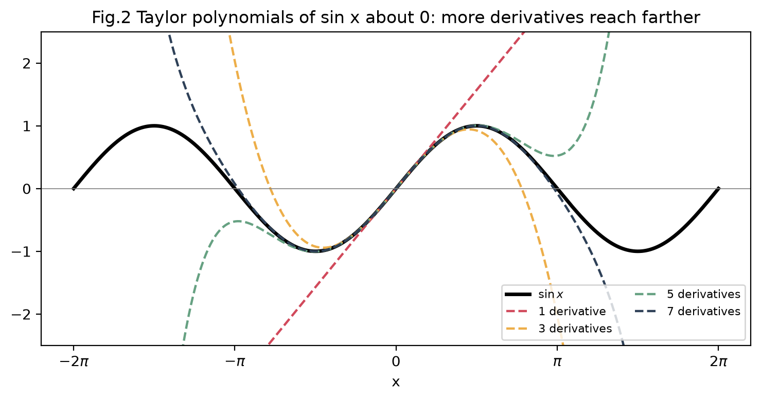

Three expansions are worth knowing by heart, all about $x = 0$ :

e^{x} = 1 + x + \frac{x^2}{2!} + \frac{x^3}{3!} + \cdots, \qquad \sin x = x - \frac{x^3}{3!} + \frac{x^5}{5!} - \cdots, \qquad \cos x = 1 - \frac{x^2}{2!} + \frac{x^4}{4!} - \cdots

(4)

Truncating after the first non-trivial term gives the small-quantity approximations used throughout chemistry: $e^{x} \approx 1 + x$ , $\sin\theta \approx \theta$ , $\cos\theta \approx 1 - \theta^2/2$ , and $(1 + x)^n \approx 1 + nx$ . Keeping the $x^2$ term of any potential energy curve near its minimum is what turns a real vibrating bond into a harmonic oscillator.

Every derivative at one point is a piece of information about the function elsewhere, and the complete set determines the function everywhere. The sum has the shape of the exponential series, which is why one writes $f(x + a) = e^{a\, d/dx} f(x)$ : exponentiating the derivative translates a function by $a$ . Later in the course the operator $d/dx$ reappears, dressed as $-i\hbar\,d/dx$ , as momentum, and this formula is the deep reason momentum and translation belong together.

Reading the first and second derivatives¶

Most of what a derivative tells you can be read off a graph without any formula. The first derivative reports the direction of the curve:

$f' > 0$ where $f$ rises, $f' < 0$ where $f$ falls, and the size of $f'$ is the steepness.
$f' = 0$ where the tangent is horizontal: a maximum, a minimum, or a flat shelf. These are the stationary points, and finding them is how one locates the most probable position, the equilibrium bond length, or the lowest energy.

The second derivative is the derivative of the slope, so it reports how the slope itself is changing, that is, how the curve bends:

$f'' > 0$ : the slope is increasing and the curve bends upward like a bowl. A stationary point there is a minimum.
$f'' < 0$ : the slope is decreasing and the curve bends downward like a dome. A stationary point there is a maximum.
$f'' = 0$ with a change of sign: an inflection point, where the bending switches direction.

The second and third bullets together are the second derivative test. The figure applies all of this to $f(x) = x^3 - 3x$ : the first derivative $3(x^2 - 1)$ vanishes at $x = \pm 1$ , the second derivative $6x$ is negative at -1 (maximum) and positive at +1 (minimum), and it changes sign at $x = 0$ (inflection).

import numpy as np
import matplotlib.pyplot as plt

x = np.linspace(-2.3, 2.3, 500)
f, fp, fpp = x**3 - 3 * x, 3 * x**2 - 3, 6 * x
UP, DOWN = '#66a182', '#d1495b'

fig, axes = plt.subplots(3, 1, figsize=(7, 8), sharex=True)
ax = axes[0]
ax.plot(x, f, 'k', lw=2.5)
ax.fill_between(x, -6, 6, where=fp > 0, color=UP, alpha=0.12)
ax.fill_between(x, -6, 6, where=fp < 0, color=DOWN, alpha=0.12)
for xc in (-1, 1):
    ax.plot([xc - 0.4, xc + 0.4], [xc**3 - 3 * xc] * 2, color='#2e4057', lw=2)
    ax.plot(xc, xc**3 - 3 * xc, 'o', color='#2e4057', ms=7)
ax.plot(0, 0, 's', color='#edae49', ms=7)
ax.text(-1, 2.6, 'maximum', ha='center', fontsize=9)
ax.text(1, -3.3, 'minimum', ha='center', fontsize=9)
ax.text(0.15, 0.4, 'inflection', fontsize=9, color='#b07d1a')
ax.text(-2.1, 3.6, 'rising', color=UP, fontsize=9)
ax.text(-0.3, 3.6, 'falling', color=DOWN, fontsize=9)
ax.text(1.5, 3.6, 'rising', color=UP, fontsize=9)
ax.set_ylim(-5, 5)
ax.set_ylabel(r'$f = x^3 - 3x$')

ax = axes[1]
ax.plot(x, fp, color='#2e4057', lw=2.5)
ax.axhline(0, color='gray', lw=0.8)
ax.plot([-1, 1], [0, 0], 'o', color='#2e4057', ms=7)
ax.fill_between(x, 0, fp, where=fp > 0, color=UP, alpha=0.25)
ax.fill_between(x, 0, fp, where=fp < 0, color=DOWN, alpha=0.25)
ax.text(-1.75, 1.5, r"$f' > 0$: rising", color=UP, fontsize=9)
ax.text(-0.6, 1.3, r"$f' < 0$: falling", color=DOWN, fontsize=9)
ax.set_ylabel(r"$f' = 3x^2 - 3$")

ax = axes[2]
ax.plot(x, fpp, color='#b07d1a', lw=2.5)
ax.axhline(0, color='gray', lw=0.8)
ax.plot(0, 0, 's', color='#edae49', ms=7)
ax.fill_between(x, 0, fpp, where=fpp > 0, color=UP, alpha=0.25)
ax.fill_between(x, 0, fpp, where=fpp < 0, color=DOWN, alpha=0.25)
ax.text(0.8, -6, r"$f'' > 0$: bends up (bowl)", color=UP, fontsize=9)
ax.text(-2.2, 6, r"$f'' < 0$: bends down (dome)", color=DOWN, fontsize=9)
ax.set_ylabel(r"$f'' = 6x$")
ax.set_xlabel('x')
fig.suptitle("Fig.3 Reading a curve from its derivatives: f' gives direction, f'' gives bending", y=0.995, fontsize=10)
plt.tight_layout()
plt.show()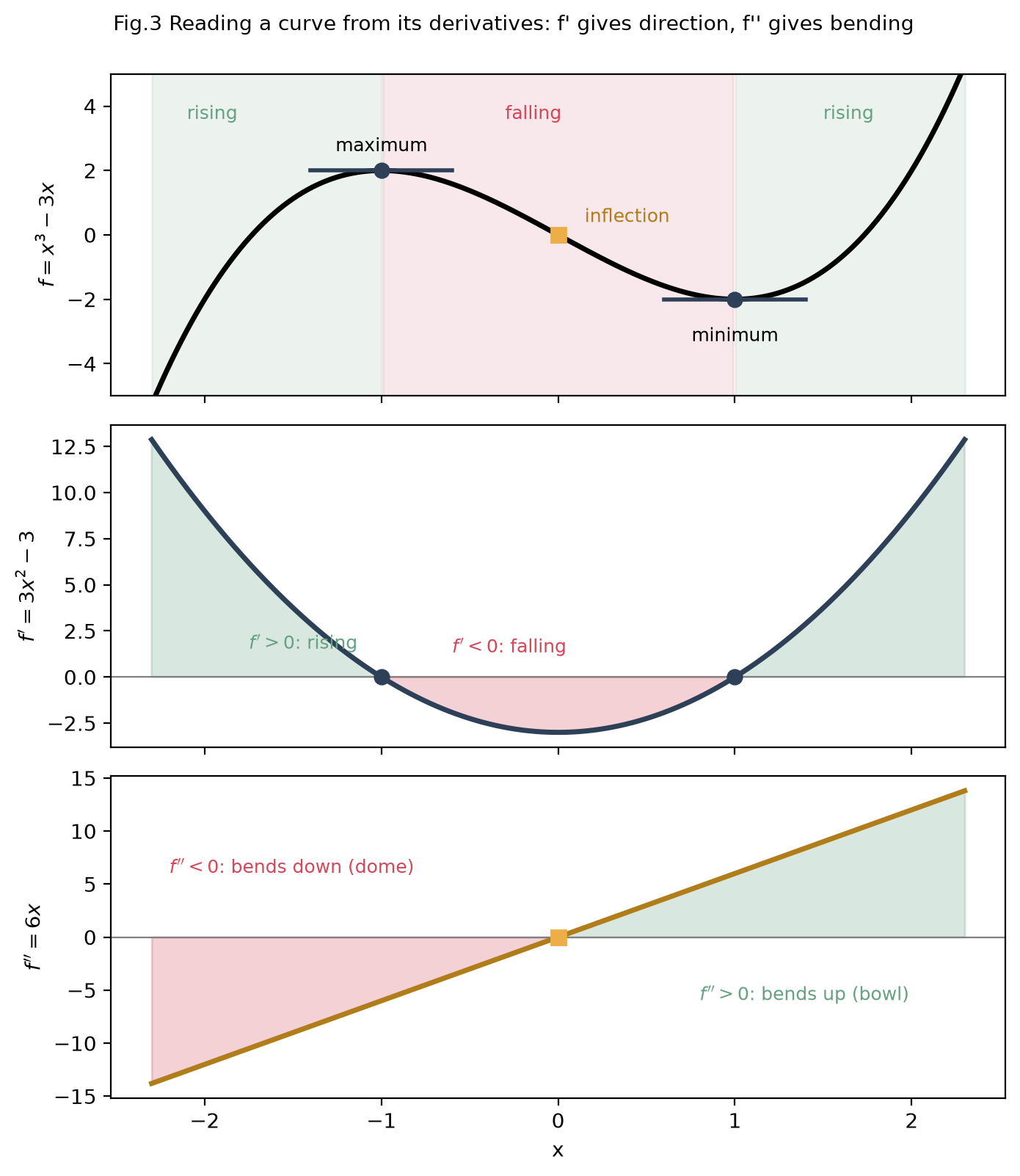

Example: locate and classify a maximum

Where is $g(x) = x\,e^{-x}$ largest for $x > 0$ , and where does it change bending?

By the product rule, $g'(x) = (1 - x)\,e^{-x}$ , which vanishes only at $x = 1$ . Differentiating again, $g''(x) = (x - 2)\,e^{-x}$ , so $g''(1) = -e^{-1} < 0$ : the curve bends downward there and $x = 1$ is a maximum, with $g(1) = 1/e$ . The second derivative changes sign at $x = 2$ , the inflection point beyond which the decaying tail bends upward toward the axis. (Curves of exactly this shape describe hydrogen orbitals along the radius, and the same two calculations locate their most probable distance from the nucleus.)

Derivatives in motion: velocity and acceleration¶

When the variable is time, the two derivatives have names everyone knows. If $x(t)$ is position, then $x'(t)$ is the velocity, how fast and in which direction, and $x''(t)$ is the acceleration, how the velocity is changing. Newton’s second law $F = m\,x''$ says that forces set the second derivative: the physics enters through the bending of the trajectory, not its slope. That is why equations of motion are second order and need two initial conditions, a position and a velocity.

The cleanest example is $x(t) = \cos t$ . Its velocity is $-\sin t$ and its acceleration is $-\cos t$ , so

x'' = -x .

(5)

The acceleration is proportional to minus the displacement: the higher the curve climbs, the harder it bends back toward zero. A function whose curvature is proportional to minus itself oscillates, and cosine and sine are exactly the functions that do this. This one relation is the harmonic oscillator, and the same structure returns in space instead of time: $\sin(kx)$ satisfies $\dfrac{d^2}{dx^2}\sin(kx) = -k^2 \sin(kx)$ , which is why sines and cosines solve the wave equation met later on this page. In quantum mechanics the curvature of a wavefunction measures its kinetic energy, so a wigglier wave means a faster particle.

import numpy as np
import matplotlib.pyplot as plt

t = np.linspace(0, 4 * np.pi, 500)
fig, ax = plt.subplots(figsize=(7.5, 3.6))
ax.plot(t, np.cos(t), 'k', lw=2.5, label=r'position $x = \cos t$')
ax.plot(t, -np.sin(t), color='#2e4057', lw=1.8, label=r"velocity $x' = -\sin t$")
ax.plot(t, -np.cos(t), color='#d1495b', lw=1.8, ls='--', label=r"acceleration $x'' = -\cos t = -x$")
ax.axhline(0, color='gray', lw=0.6)
ax.set_xticks([0, np.pi, 2 * np.pi, 3 * np.pi, 4 * np.pi])
ax.set_xticklabels(['0', r'$\pi$', r'$2\pi$', r'$3\pi$', r'$4\pi$'])
ax.set_xlabel('t')
ax.set_ylim(-1.8, 1.8)
ax.legend(fontsize=8, loc='upper right', ncol=3)
ax.set_title('Fig.4 Cosine motion: the acceleration is the mirror image of the position')
plt.tight_layout()
plt.show()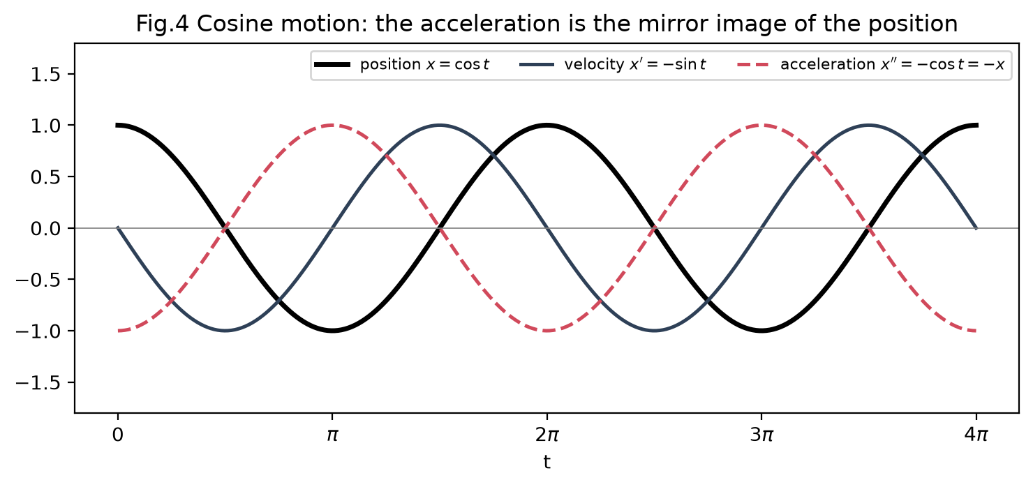

Rules of differentiation¶

Six Key Derivative Rules

Constant multiple: if $h(x) = c\, f(x)$ , then
$\frac{dh}{dx} = c\, \frac{df}{dx}$
(6)
Sum and difference: if $h(x) = f(x) \pm g(x)$ , then
$\frac{dh}{dx} = \frac{df}{dx} \pm \frac{dg}{dx}$
(7)
Power rule:
$\frac{d}{dx}\, x^n = n\, x^{n-1}$
(8)
Product rule: if $h(x) = f(x)\, g(x)$ , then
$\frac{dh}{dx} = \frac{df}{dx}\, g + f\, \frac{dg}{dx}$
(9)
Equivalently, $h'(x) = f'(x)g(x) + f(x)g'(x)$ .
Quotient rule: if $h(x) = \dfrac{f(x)}{g(x)}$ , then
$\frac{dh}{dx} = \frac{f'(x)\,g(x) - f(x)\,g'(x)}{g(x)^2}$
(10)
Chain rule: if $h(x) = f(g(x))$ , then
$\frac{dh}{dx} = \frac{df}{dg} \cdot \frac{dg}{dx}$
(11)
Equivalently, $h'(x) = f'(g(x))\, g'(x)$ .

Bonus, used everywhere in approximations: the linear approximation $f(x) \approx f(a) + f'(a)(x - a)$ .

Example: a product with a composition inside¶

Differentiate $f(x) = x^2 e^{-\alpha x^2}$ . Attempt this before peeking at the solution. (Functions of exactly this shape describe vibrating molecules later in the course.)

Solution

Split into $x^2$ times $e^{-\alpha x^2}$ and apply the product rule:

\frac{df}{dx} = \underbrace{2x}_{(x^2)'}\, e^{-\alpha x^2} + x^2\, \underbrace{(-2\alpha x)\, e^{-\alpha x^2}}_{(e^{-\alpha x^2})' \text{ by the chain rule}} = 2x\, (1 - \alpha x^2)\, e^{-\alpha x^2}.

(12)

The chain rule handled the inner function $g(x) = -\alpha x^2$ inside the exponential. Setting $f'(x) = 0$ gives $x = 0$ and $x = \pm 1/\sqrt{\alpha}$ : a minimum at the origin flanked by two maxima.

The chain rule is the one you will use most

Almost every function you will meet in this course is a composition: $e^{-x^2}$ , $\sin(kx)$ , $e^{ikx}$ . Each needs the chain rule. For $\dfrac{d}{dx} e^{-\alpha x^2}$ , take the outer derivative $e^{u}$ times the inner derivative $-2\alpha x$ , giving $-2\alpha x\, e^{-\alpha x^2}$ .

Table of common derivatives¶

Function $f(x)$	Derivative $f'(x)$	Function $f(x)$	Derivative $f'(x)$
$c$	0	$x^n$	$nx^{n-1}$
$e^{x}$	$e^{x}$	$\ln x$	$\dfrac{1}{x}$
$\sin x$	$\cos x$	$\cos x$	$-\sin x$
$\tan x$	$\sec^2 x$	$e^{ax}$	$a\,e^{ax}$
$\arcsin x$	$\dfrac{1}{\sqrt{1-x^2}}$	$\arctan x$	$\dfrac{1}{1+x^2}$

A few limits underlie these results: $\displaystyle\lim_{\theta\to 0}\frac{\sin\theta}{\theta}=1$ , $\displaystyle\lim_{\theta\to 0}\frac{\cos\theta-1}{\theta}=0$ , and the definition $\displaystyle\lim_{h\to 0}\frac{e^{h}-1}{h}=1$ , which is exactly what makes $e^{x}$ its own derivative.

Solution

$f'(x) = -2ax\, e^{-ax^2}$ (chain rule), and the product plus chain rules give $f''(x) = (4a^2x^2 - 2a)\, e^{-ax^2}$ . The first derivative vanishes only at $x = 0$ , where $f'' = -2a < 0$ : the peak is a maximum. Setting $f'' = 0$ gives $x = \pm 1/\sqrt{2a}$ : the inflection points where the bell curve changes from bending down to bending up. Remember this pair of points; when the Gaussian returns as a vibrational state they turn out to be the classical turning points.

import numpy as np
import matplotlib.pyplot as plt

x = np.linspace(-3, 3, 500)
g = np.exp(-x**2)
fig, ax = plt.subplots(figsize=(7.5, 4))
ax.plot(x, g, 'k', lw=2.5, label=r'$f = e^{-x^2}$')
ax.plot(x, -2 * x * g, color='#2e4057', lw=1.8, label=r"$f' = -2x\,e^{-x^2}$")
ax.plot(x, (4 * x**2 - 2) * g, color='#d1495b', lw=1.8, ls='--', label=r"$f'' = (4x^2 - 2)\,e^{-x^2}$")
ax.axhline(0, color='gray', lw=0.6)
xi = 1 / np.sqrt(2)
for xc in (-xi, xi):
    ax.axvline(xc, color='#b07d1a', lw=1, ls=':')
    ax.plot(xc, np.exp(-xc**2), 's', color='#edae49', ms=7)
ax.plot(0, 1, 'o', color='#2e4057', ms=7)
ax.text(0, 1.1, r"peak: $f' = 0$, $f'' < 0$", ha='center', fontsize=9)
ax.text(xi + 0.08, 0.72, r"inflection: $f'' = 0$", fontsize=9, color='#b07d1a')
ax.set_ylim(-2.3, 1.4)
ax.set_xlabel('x')
ax.legend(fontsize=8, loc='lower right')
ax.set_title('Fig.5 The Gaussian with its first two derivatives (a = 1)')
plt.tight_layout()
plt.show()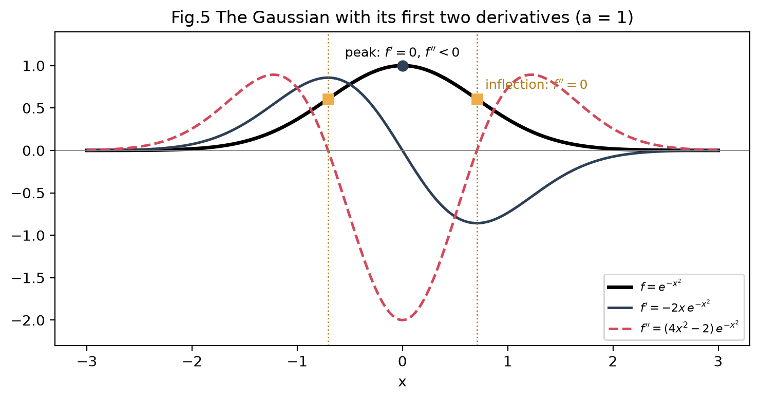

Functions of several variables¶

Partial derivatives¶

Most quantities in chemistry depend on more than one variable. The pressure of an ideal gas depends on both volume and temperature, $P(V,T) = nRT/V$ , and the displacement of a plucked guitar string depends on where you look and when, $u(x,t)$ . Graphically, a function of two variables $f(x,y)$ is a surface over the $xy$ plane, and a surface has no single slope: it can be steep along $x$ and nearly flat along $y$ .

The fix is to vary one variable at a time. The partial derivative of $f$ with respect to $x$ is the ordinary derivative along $x$ with every other variable frozen:

Nothing new is needed to compute one: treat the other variables as constants and apply the rules of the previous section. Geometrically, slicing the surface with the plane $y = y_0$ leaves an ordinary curve, and $\partial f/\partial x$ is the slope of that curve.

import numpy as np
import matplotlib.pyplot as plt

f = lambda x, y: 4 - x**2 - y**2 / 4
fx = lambda x, y: -2 * x
fy = lambda x, y: -y / 2
x0, y0 = 1.0, 1.0

X, Y = np.meshgrid(np.linspace(-2, 2, 60), np.linspace(-3, 3, 60))
fig = plt.figure(figsize=(7.5, 5.5))
ax = fig.add_subplot(111, projection='3d')
ax.plot_surface(X, Y, f(X, Y), color='lightgray', alpha=0.35, linewidth=0)

xs = np.linspace(-2, 2, 100)
ys = np.linspace(-3, 3, 100)
ax.plot(xs, np.full_like(xs, y0), f(xs, y0), color='#d1495b', lw=2.5,
        label=r'slice $y = 1$: slope is $\partial f/\partial x$')
ax.plot(np.full_like(ys, x0), ys, f(x0, ys), color='#66a182', lw=2.5,
        label=r'slice $x = 1$: slope is $\partial f/\partial y$')

tx = np.array([x0 - 0.8, x0 + 0.8])
ax.plot(tx, np.full_like(tx, y0), f(x0, y0) + fx(x0, y0) * (tx - x0), '--', color='#d1495b', lw=1.5)
ty = np.array([y0 - 1.2, y0 + 1.2])
ax.plot(np.full_like(ty, x0), ty, f(x0, y0) + fy(x0, y0) * (ty - y0), '--', color='#66a182', lw=1.5)
ax.scatter([x0], [y0], [f(x0, y0)], color='k', s=40)

ax.set_xlabel('x')
ax.set_ylabel('y')
ax.set_zlabel('f(x, y)')
ax.view_init(elev=25, azim=-60)
ax.legend(loc='upper left', fontsize=8)
ax.set_title('Fig.6 Partial derivatives are slopes of slices through the surface')
plt.tight_layout()
plt.show()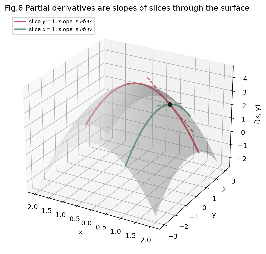

For the hill $f(x,y) = 4 - x^2 - y^2/4$ in the figure, $\partial f/\partial x = -2x$ and $\partial f/\partial y = -y/2$ . At the marked point $(1, 1)$ the surface drops four times faster along $x$ than along $y$ , which is why the red tangent is steeper than the green one.

Second and mixed partial derivatives¶

Differentiating twice along the same variable gives $\dfrac{\partial^2 f}{\partial x^2}$ , written $f_{xx}$ ; differentiating once along each gives the mixed partial $\dfrac{\partial^2 f}{\partial y\,\partial x}$ , written $f_{xy}$ . For every smooth function the order does not matter:

\frac{\partial^2 f}{\partial y\,\partial x} = \frac{\partial^2 f}{\partial x\,\partial y}.

(14)

For the example above, $f_{xy} = 2x + \cos(xy) - xy\sin(xy)$ whichever variable you differentiate first. This innocent-looking equality is the origin of the Maxwell relations of thermodynamics.

The chain rule on a sliding shape¶

The most important partial-derivative calculation in this course involves a function of the single combination $x - vt$ . Take any smooth profile $f$ and a constant $v$ , and define

u(x,t) = f(x - vt).

(15)

At $t = 0$ the graph of $u$ is just the graph of $f$ ; at a later time the same shape has moved a distance $vt$ to the right. So $u$ describes a shape sliding at speed $v$ without changing form. Its partial derivatives follow from the chain rule with the inner function $s = x - vt$ , for which $\partial s/\partial x = 1$ and $\partial s/\partial t = -v$ :

\frac{\partial u}{\partial x} = f'(s)\cdot 1 = f'(s), \qquad \frac{\partial u}{\partial t} = f'(s)\cdot(-v) = -v\,f'(s).

(16)

Differentiate once more and every factor of $v$ appears again:

\frac{\partial^2 u}{\partial x^2} = f''(s), \qquad \frac{\partial^2 u}{\partial t^2} = v^2 f''(s).

(17)

Eliminating $f''$ between the two lines gives a relation that holds for every sliding shape, whatever $f$ is:

\frac{\partial^2 u}{\partial x^2} = \frac{1}{v^2}\,\frac{\partial^2 u}{\partial t^2}.

(18)

This is the classical wave equation. Here it emerged from calculus alone; in the waves lecture the same equation gets its physical meaning, and the shorthand $u_{xx}$ and $u_{tt}$ used there is the subscript notation introduced above. The same steps with $f(x + vt)$ give a shape sliding to the left and the identical relation, since $v$ enters only as $v^2$ .

Solution

$\left(\partial P/\partial V\right)_T = -nRT/V^2$ (power rule in $V$ with $T$ frozen) and $\left(\partial P/\partial T\right)_V = nR/V$ (linear in $T$ with $V$ frozen). Hence

dP = -\frac{nRT}{V^2}\,dV + \frac{nR}{V}\,dT.

(19)

This total differential adds up the change coming from each variable separately, one partial derivative per variable. It is the everyday tool of thermodynamics.

Integration¶

The integral as accumulated area¶

A definite integral measures the net area between a curve and the $x$ axis. We approximate that area with a Riemann sum of $n$ rectangles and let $n\to\infty$ :

The plot shows the rectangles filling the area under $f(x)=x^2$ on $[0,2]$ as $n$ grows from coarse to fine. The exact area is $\int_0^2 x^2\,dx = 8/3 \approx 2.667$ .

import numpy as np
import matplotlib.pyplot as plt

f = lambda x: x**2
a, b = 0, 2
xs = np.linspace(a, b, 400)

fig, axes = plt.subplots(1, 3, figsize=(11, 3.6), sharey=True)
for ax, n in zip(axes, [4, 8, 32]):
    edges = np.linspace(a, b, n + 1)
    mids = 0.5 * (edges[:-1] + edges[1:])   # midpoint rule
    dx = (b - a) / n
    approx = np.sum(f(mids) * dx)
    ax.bar(mids, f(mids), width=dx, align='center',
           color='#66a182', edgecolor='white', alpha=0.7)
    ax.plot(xs, f(xs), 'k', lw=2)
    ax.set_title(f'n = {n},  sum = {approx:.3f}', fontsize=10)
    ax.set_xlabel('x')
axes[0].set_ylabel('f(x)')
plt.suptitle('Fig.7 Riemann sums approaching the exact area 8/3 = 2.667 as n grows', y=1.04)
plt.tight_layout()
plt.show()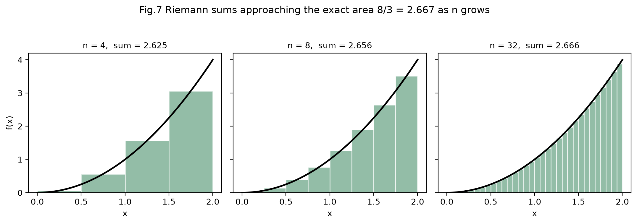

We can watch that convergence numerically:

import numpy as np

f = lambda x: x**2
a, b = 0.0, 2.0
for n in [4, 16, 64, 256, 1024]:
    x = np.linspace(a, b, n + 1)
    mids = 0.5 * (x[:-1] + x[1:])
    approx = np.sum(f(mids) * (b - a) / n)
    print(f"n = {n:5d}   Riemann sum = {approx:.5f}")

exact = 8 / 3
print(f"\nexact value  = {exact:.5f}")

n =     4   Riemann sum = 2.62500
n =    16   Riemann sum = 2.66406
n =    64   Riemann sum = 2.66650
n =   256   Riemann sum = 2.66666
n =  1024   Riemann sum = 2.66667

exact value  = 2.66667

Antiderivatives and the fundamental theorem¶

An antiderivative $F$ of $f$ satisfies $F'(x)=f(x)$ . Because the derivative of a constant is zero, antiderivatives come as a family $F(x)+C$ . The fundamental theorem of calculus ties the two halves of the subject together:

This is why we rarely compute Riemann sums by hand: finding an antiderivative turns an infinite sum into a single subtraction.

Table of indefinite integrals¶

Function $f(x)$	Antiderivative $F(x)$	Function $f(x)$	Antiderivative $F(x)$
$x^n\ (n\neq -1)$	$\dfrac{x^{n+1}}{n+1} + C$	$\dfrac{1}{x}$	$\ln\lvert x \rvert + C$
$e^{x}$	$e^{x} + C$	$e^{ax}$	$\dfrac{1}{a}e^{ax} + C$
$\sin x$	$-\cos x + C$	$\cos x$	$\sin x + C$
$\dfrac{1}{x^2 + a^2}$	$\dfrac{1}{a}\arctan\!\left(\dfrac{x}{a}\right) + C$	$\dfrac{1}{\sqrt{a^2-x^2}}$	$\arcsin\!\left(\dfrac{x}{a}\right) + C$

Useful properties: reversing the limits flips the sign, $\int_a^a f\,dx = 0$ , and integrals are linear, $\int (cf \pm g)\,dx = c\int f\,dx \pm \int g\,dx$ . For symmetric limits, an even function gives $\int_{-a}^{a} f\,dx = 2\int_0^a f\,dx$ while an odd function gives $\int_{-a}^{a} f\,dx = 0$ , a shortcut that kills many quantum-mechanical integrals on sight.

Techniques of integration¶

Integration by parts is the reverse of the product rule, and it is the standard tool for integrals like $\int x\,e^{-x}\,dx$ or $\int x\sin x\,dx$ that appear constantly in expectation-value calculations.

For products of sines and cosines, the power-reduction and product-to-sum identities do the work:

\sin^2 x = \tfrac{1}{2}(1-\cos 2x), \qquad \cos^2 x = \tfrac{1}{2}(1+\cos 2x),

(24)

\sin A\sin B = \tfrac{1}{2}\big[\cos(A-B)-\cos(A+B)\big], \qquad \cos A\cos B = \tfrac{1}{2}\big[\cos(A-B)+\cos(A+B)\big].

(25)

These are exactly the integrals that enforce orthogonality of particle-in-a-box wavefunctions.

Solution

(a) With $\sin^2 u = \tfrac{1}{2}(1 - \cos 2u)$ , the cosine integrates to zero over full half-periods, leaving $L/2$ . That is why box wavefunctions carry the prefactor $\sqrt{2/L}$ .

(b) Integrate by parts twice (or recognize $\Gamma(3) = 2!$ ): the answer is 2. In general $\int_0^\infty x^n e^{-x} dx = n!$ , the workhorse of radial hydrogen integrals.

Problems¶

Problem 1: Differentiate a Gaussian¶

Differentiate $f(x) = e^{-\alpha x^2}$ with respect to $x$ .

Solution

Chain rule with outer $e^{u}$ and inner $u = -\alpha x^2$ :

f'(x) = e^{-\alpha x^2}\cdot(-2\alpha x) = -2\alpha x\,e^{-\alpha x^2}.

(26)

Note the derivative is zero at $x=0$ , the peak of the Gaussian.

Problem 2: Product and chain together¶

Differentiate $g(x) = x\sin(kx)$ .

Solution

Product rule, and the chain rule on $\sin(kx)$ :

g'(x) = \sin(kx) + x\cdot k\cos(kx).

(27)

Problem 3: A normalization integral¶

Evaluate $\displaystyle\int_0^{L} \sin^2\!\left(\frac{\pi x}{L}\right)dx$ .

Solution

Use $\sin^2\theta = \tfrac{1}{2}(1-\cos 2\theta)$ with $\theta = \pi x/L$ :

\int_0^L \tfrac{1}{2}\left(1 - \cos\tfrac{2\pi x}{L}\right)dx = \tfrac{1}{2}\left[x - \tfrac{L}{2\pi}\sin\tfrac{2\pi x}{L}\right]_0^L = \frac{L}{2}.

(28)

The sine term vanishes at both limits. This is the integral behind the particle-in-a-box normalization constant $\sqrt{2/L}$ .

Problem 4: Integration by parts¶

Evaluate $\displaystyle\int_0^{\infty} x\,e^{-x}\,dx$ .

Solution

Let $u = x$ , $dv = e^{-x}dx$ , so $du = dx$ and $v = -e^{-x}$ :

\int_0^\infty x\,e^{-x}\,dx = \big[-x e^{-x}\big]_0^\infty + \int_0^\infty e^{-x}\,dx = 0 + 1 = 1.

(29)

Problem 5: Symmetry shortcut¶

Without computing an antiderivative, evaluate $\displaystyle\int_{-a}^{a} x\,e^{-x^2}\,dx$ .

Solution

The integrand is odd: replacing $x\to -x$ flips its sign. The integral over symmetric limits is therefore 0.

Problem 6: Mixed partial derivatives¶

For $f(x,y) = x^3 y^2 + e^{xy}$ find $\partial f/\partial x$ and $\partial f/\partial y$ , then verify that the two mixed second derivatives agree.

Solution

With $y$ frozen, $\dfrac{\partial f}{\partial x} = 3x^2 y^2 + y\,e^{xy}$ ; with $x$ frozen, $\dfrac{\partial f}{\partial y} = 2x^3 y + x\,e^{xy}$ .

Differentiating the first result with respect to $y$ and the second with respect to $x$ :

\frac{\partial^2 f}{\partial y\,\partial x} = 6x^2 y + e^{xy} + xy\,e^{xy}, \qquad \frac{\partial^2 f}{\partial x\,\partial y} = 6x^2 y + e^{xy} + xy\,e^{xy}.

(30)

They match, as they must for any smooth function.

Problem 7: Verify a Riemann sum numerically¶

Modify the Riemann-sum code above to estimate $\int_0^{\pi}\sin x\,dx$ and compare with the exact value 2.

Problem 8: Chain rule on a plane wave¶

Differentiate $\psi(x) = e^{ikx}$ with respect to $x$ , and again to find $\psi''(x)$ .

Problem 9: A Gamma-function integral¶

Evaluate $\displaystyle\int_0^{\infty} x^2\,e^{-x}\,dx$ using integration by parts twice.

Problem 10: A standing shape¶

Show that $u(x,t) = \sin(kx)\cos(\omega t)$ satisfies $\dfrac{\partial^2 u}{\partial x^2} = \dfrac{k^2}{\omega^2}\,\dfrac{\partial^2 u}{\partial t^2}$ . Compare with the relation obeyed by the sliding shape $f(x - vt)$ and read off the speed $v$ .