Trigonometry and Complex Numbers - Quantum Mechanics for Chemistry

What you will learn

Trigonometry as geometry on the unit circle. Sine and cosine are the coordinates of a point rotating around a circle of radius one.
The key identities. The Pythagorean identity, angle-sum formulas, and power-reduction formulas that recur throughout quantum mechanics.
Complex numbers as 2D numbers. A complex number carries a real and an imaginary part and lives in a plane.
Euler’s formula. $e^{i\phi} = \cos\phi + i\sin\phi$ fuses trigonometry and exponentials into one object and is the single most useful identity in the course.
Polar form, conjugation, and rotation. Multiplying complex numbers rotates and scales them, and the conjugate reflects across the real axis.
Waves as rotating phases. A cosine wave is the real part of $e^{i(kx - \omega t)}$ , which turns derivatives into multiplications and the addition of waves into the addition of arrows.

Trigonometry and complex numbers are two views of the same thing: rotation in a plane. Waves, oscillations, and quantum phases all live here, and Euler’s formula is the bridge that connects them. We treat them together because in quantum mechanics you almost never use one without the other.

Trigonometry¶

Sine and cosine on the unit circle¶

Take a point on a circle of radius 1 and rotate it counterclockwise by an angle $\theta$ (measured in radians, where a full turn is $2\pi$ ). Its coordinates are, by definition,

x = \cos\theta, \qquad y = \sin\theta.

(1)

Cosine is the horizontal coordinate, sine the vertical one, and the tangent $\tan\theta = \sin\theta/\cos\theta$ is the slope of the radius.

import numpy as np
import matplotlib.pyplot as plt

theta = np.deg2rad(50)
t = np.linspace(0, 2 * np.pi, 400)

fig, ax = plt.subplots(figsize=(5.5, 5.5))
ax.plot(np.cos(t), np.sin(t), 'k', lw=1.5)           # unit circle
ax.plot([0, np.cos(theta)], [0, np.sin(theta)], color='#2e4057', lw=2)  # radius
ax.plot([np.cos(theta), np.cos(theta)], [0, np.sin(theta)], color='#66a182', lw=2, label=r'$\sin\theta$')
ax.plot([0, np.cos(theta)], [0, 0], color='#d1495b', lw=2, label=r'$\cos\theta$')
ax.plot(np.cos(theta), np.sin(theta), 'ko', ms=6)

ax.annotate(r'$(\cos\theta,\ \sin\theta)$', (np.cos(theta), np.sin(theta)),
            textcoords='offset points', xytext=(8, 8), fontsize=11)
ax.axhline(0, color='gray', lw=0.6)
ax.axvline(0, color='gray', lw=0.6)
ax.set_aspect('equal')
ax.set_xlim(-1.3, 1.5)
ax.set_ylim(-1.3, 1.3)
ax.legend(loc='lower left', fontsize=10)
ax.set_title(r'Fig.1 Sine and cosine as coordinates on the unit circle ($\theta=50^\circ$)')
plt.tight_layout()
plt.show()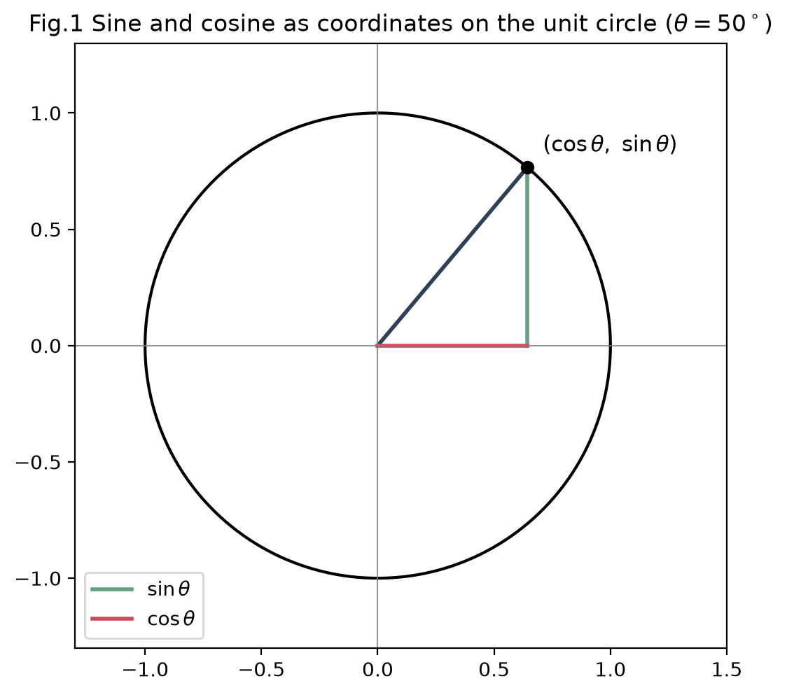

As $\theta$ runs around the circle, the two coordinates trace out the familiar waves: cosine starts at 1, sine starts at 0, and each is the other shifted by a quarter turn.

import numpy as np
import matplotlib.pyplot as plt

t = np.linspace(0, 2 * np.pi, 400)
fig, ax = plt.subplots(figsize=(7, 3.2))
ax.plot(t, np.cos(t), color='#d1495b', lw=2, label=r'$\cos\theta$')
ax.plot(t, np.sin(t), color='#66a182', lw=2, label=r'$\sin\theta$')
ax.axhline(0, color='gray', lw=0.6)
ax.set_xticks([0, np.pi / 2, np.pi, 3 * np.pi / 2, 2 * np.pi])
ax.set_xticklabels(['0', r'$\pi/2$', r'$\pi$', r'$3\pi/2$', r'$2\pi$'])
ax.set_xlabel(r'$\theta$ (radians)')
ax.legend(fontsize=10, loc='upper right')
ax.set_title('Fig.2 Cosine and sine as functions of the angle, offset by a quarter turn')
plt.tight_layout()
plt.show()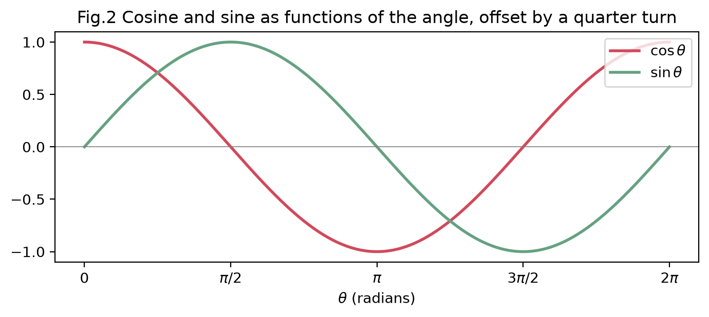

Key identities¶

Because the point lies on a unit circle, its coordinates always satisfy the Pythagorean identity:

The identities you will reach for most often are the angle-sum and power-reduction formulas:

\sin(A \pm B) = \sin A\cos B \pm \cos A\sin B, \qquad \cos(A \pm B) = \cos A\cos B \mp \sin A\sin B,

(3)

\sin^2\theta = \tfrac{1}{2}(1-\cos 2\theta), \qquad \cos^2\theta = \tfrac{1}{2}(1+\cos 2\theta).

(4)

For small angles (in radians), the first terms of the Taylor series give the approximations $\sin\theta \approx \theta$ and $\cos\theta \approx 1 - \tfrac{1}{2}\theta^2$ , which are what let us linearize a pendulum or a vibrating bond near equilibrium.

Rather than memorize the whole table of identities, it is easier to derive them from Euler’s formula, which we build next.

Complex numbers¶

Complex numbers live in 2D¶

A complex number $z$ is a two-dimensional number: it needs two components for its full specification. They arise the moment we ask for the roots of a simple polynomial. The equation

x^2 + 1 = 0 \quad\Longrightarrow\quad x_{1,2} = \pm\sqrt{-1} = \pm i

(5)

has no real solution, so we extend the real line $\mathbb{R}$ into the complex plane $\mathbb{C}$ by introducing the imaginary unit $i$ , defined solely by

i^2 = -1.

(6)

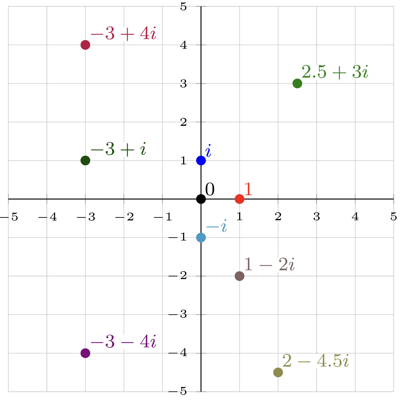
Complex numbers live in 2D — Fig.3 A complex number needs a real and an imaginary component to be fully specified, so it lives in a plane.

The quadratic formula and the discriminant

For $ax^2 + bx + c = 0$ the roots are $x = \dfrac{-b \pm \sqrt{b^2 - 4ac}}{2a}$ . The discriminant $\Delta = b^2 - 4ac$ decides their nature: $\Delta > 0$ gives two real roots, $\Delta = 0$ a repeated real root, and $\Delta < 0$ two complex conjugate roots.

Cartesian representation¶

Polar representation and Euler’s formula¶

Instead of horizontal and vertical parts, we can locate $z$ by its distance from the origin $r$ and its angle $\phi$ . From the unit-circle picture, $x = r\cos\phi$ and $y = r\sin\phi$ , so

z = x + iy = r(\cos\phi + i\sin\phi).

(8)

The magic step is Euler’s formula, which collapses the parenthesis into an exponential:

Proof of Euler’s formula from Taylor series

Expand $e^{ix}$ and collect powers of $i$ :

e^{ix} = 1 + ix - \frac{x^2}{2!} - i\frac{x^3}{3!} + \frac{x^4}{4!} + \cdots = \left(1 - \frac{x^2}{2!} + \cdots\right) + i\left(x - \frac{x^3}{3!} + \cdots\right).

(10)

The two series are exactly $\cos x$ and $\sin x$ , so $e^{ix} = \cos x + i\sin x$ .

The plot below shows why polar form is natural: the same complex number is one dot in the plane, described equally well by $(x, y)$ or by $(r, \phi)$ .

import numpy as np
import matplotlib.pyplot as plt

z = 2 + 1.5j
r, phi = np.abs(z), np.angle(z)

fig, ax = plt.subplots(figsize=(5.5, 5))
ax.annotate('', xy=(z.real, z.imag), xytext=(0, 0),
            arrowprops=dict(arrowstyle='->', color='#2e4057', lw=2))
arc = np.linspace(0, phi, 60)
ax.plot(0.6 * np.cos(arc), 0.6 * np.sin(arc), color='#d1495b', lw=1.5)
ax.plot([0, z.real], [z.imag, z.imag], '--', color='gray', lw=1)
ax.plot([z.real, z.real], [0, z.imag], '--', color='gray', lw=1)

ax.text(z.real + 0.1, z.imag + 0.1, fr'$z = {z.real:.0f}+{z.imag:.1f}i = {r:.2f}\,e^{{i\phi}}$', fontsize=11)
ax.text(0.7, 0.15, r'$\phi$', color='#d1495b', fontsize=13)
ax.text(z.real / 2, -0.25, r'$x=r\cos\phi$', color='gray', fontsize=9, ha='center')
ax.text(z.real + 0.05, z.imag / 2, r'$y=r\sin\phi$', color='gray', fontsize=9)

ax.axhline(0, color='black', lw=0.8)
ax.axvline(0, color='black', lw=0.8)
ax.set_xlim(-0.6, 3)
ax.set_ylim(-0.6, 2.4)
ax.set_aspect('equal')
ax.set_xlabel('Real')
ax.set_ylabel('Imaginary')
ax.set_title('Fig.4 The same number in Cartesian (x, y) and polar (r, phi) form')
plt.tight_layout()
plt.show()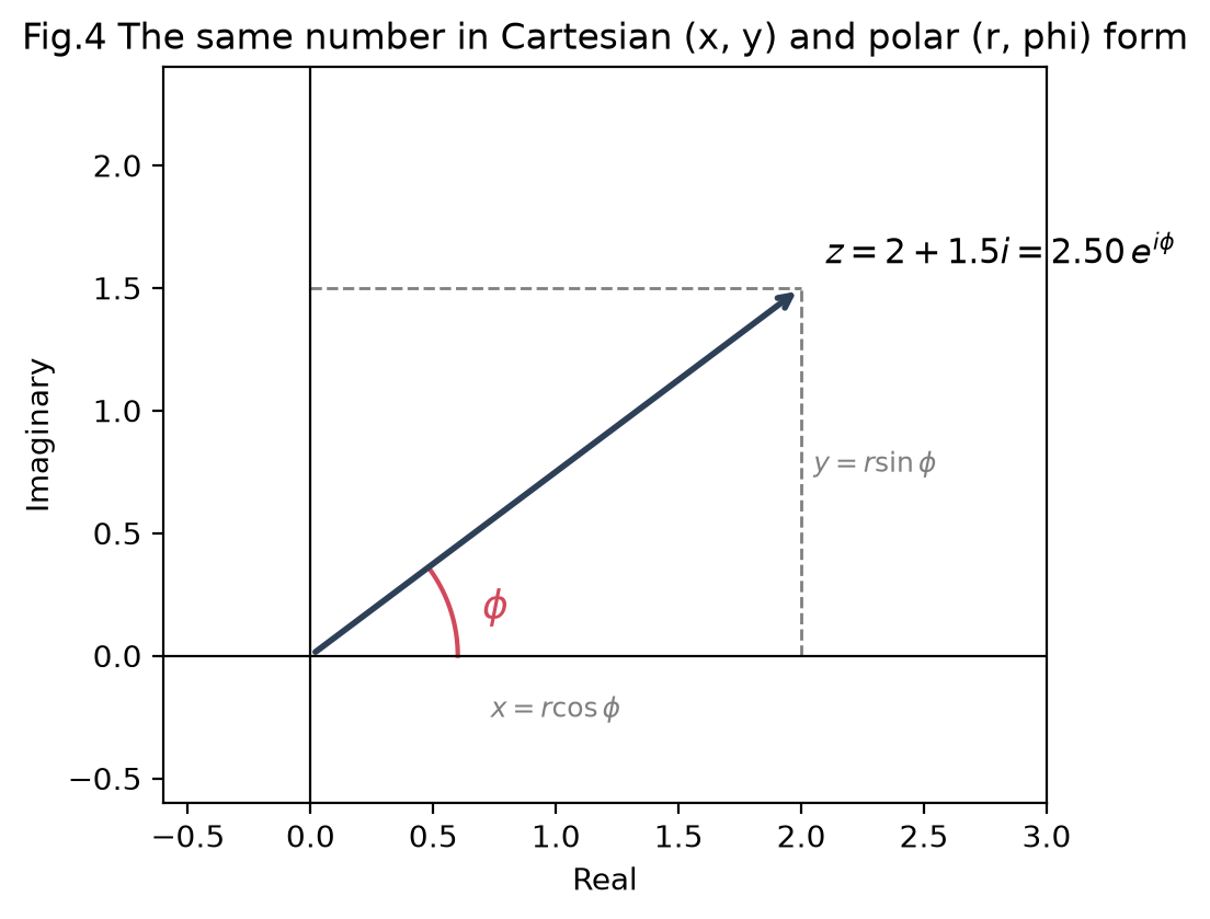

Multiplication is rotation¶

In polar form, multiplication becomes almost trivial: magnitudes multiply and angles add.

(r_1 e^{i\phi_1})(r_2 e^{i\phi_2}) = r_1 r_2\, e^{i(\phi_1 + \phi_2)}.

(12)

Now read that formula geometrically. The number $e^{i\phi} = \cos\phi + i\sin\phi$ has magnitude

|e^{i\phi}| = \sqrt{\cos^2\phi + \sin^2\phi} = 1,

(13)

so it sits on the unit circle. Multiplying any $z$ by it therefore cannot stretch or shrink $z$ at all:

The cleanest special case is $i = e^{i\pi/2}$ : multiplying by $i$ is a quarter-turn counterclockwise. Do it four times and you are home, which is the geometric meaning of $i^4 = 1$ :

z0 = 1.6 + 0.6j
pts = [z0, 1j*z0, -z0, -1j*z0]
labels = [r"$z$", r"$iz$", r"$i^2z=-z$", r"$i^3z=-iz$"]
colors = ["orange", "#3d81f6", "#004d40", "#d81b60"]

fig, ax = plt.subplots(figsize=(5.5, 5.5))
th = np.linspace(0, 2*np.pi, 200)
R = abs(z0)
ax.plot(R*np.cos(th), R*np.sin(th), "--", color="gray", lw=1)
for w, lab, c in zip(pts, labels, colors):
    ax.annotate("", xy=(w.real, w.imag), xytext=(0, 0),
                arrowprops=dict(arrowstyle="->", color=c, lw=2.5))
    ax.text(w.real*1.15, w.imag*1.15, lab, color=c, fontsize=13, ha="center")
for k in range(4):
    a0, a1 = np.angle(pts[k]), np.angle(pts[k]) + np.pi/2
    arc = np.linspace(a0 + 0.15, a1 - 0.15, 40)
    ax.plot(0.45*np.cos(arc), 0.45*np.sin(arc), color="gray", lw=1)
ax.axhline(0, color="black", lw=0.7)
ax.axvline(0, color="black", lw=0.7)
ax.set_xlim(-2.4, 2.4); ax.set_ylim(-2.4, 2.4)
ax.set_aspect("equal")
ax.set_xlabel("Real"); ax.set_ylabel("Imaginary")
ax.set_title("Fig.5 Multiplying by i is a quarter-turn: four turns return z to itself")
plt.tight_layout()
plt.show()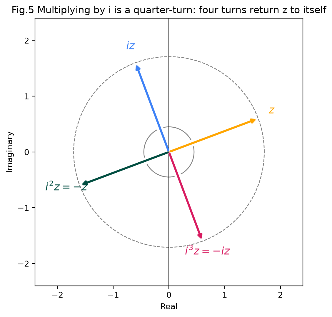

Try it yourself: dial the angle and watch $z$ swing around the circle while its length refuses to change. Negative $\phi$ turns it clockwise.

This rotating phase is the single most reused picture in quantum mechanics: every stationary state carries the factor $e^{-iEt/\hbar}$ , a clock hand turning clockwise at rate $E/\hbar$ . When the time dependence of wavefunctions looks abstract, come back to this circle.

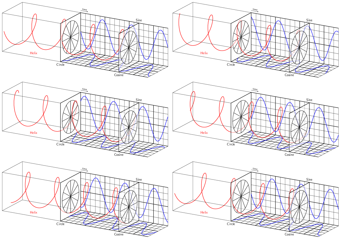
Euler's formula traced as a helix — Fig.6 As $t$ increases, $e^{i\omega t}$ traces a helix. Its shadow on one wall is $\cos\omega t$ and on the other is $\sin\omega t$ , so a single rotating phase carries both waves at once.

The complex conjugate¶

The conjugate flips the sign of the imaginary part, reflecting $z$ across the real axis:

Multiplying a number by its conjugate rotates it back onto the real axis and returns a non-negative real number, the squared magnitude:

|z|^2 = \bar{z}\,z = (x - iy)(x + iy) = x^2 + y^2 = r^2.

(16)

This is exactly the operation that turns a quantum amplitude $\psi$ into a probability density $|\psi|^2 = \psi^*\psi$ .

Taking sums and differences of $z$ and $\bar{z}$ recovers the trig functions as exponentials, a substitution that simplifies countless integrals:

\cos\phi = \frac{e^{i\phi} + e^{-i\phi}}{2}, \qquad \sin\phi = \frac{e^{i\phi} - e^{-i\phi}}{2i}.

(17)

Deriving the angle-sum identities from Euler’s formula

Expand $e^{i(\omega+\theta)} = e^{i\omega}e^{i\theta}$ and match real and imaginary parts:

\cos(\omega+\theta) + i\sin(\omega+\theta) = (\cos\omega + i\sin\omega)(\cos\theta + i\sin\theta).

(18)

Multiplying out the right side and equating parts gives both angle-sum identities at once:

\cos(\omega+\theta) = \cos\omega\cos\theta - \sin\omega\sin\theta, \qquad \sin(\omega+\theta) = \sin\omega\cos\theta + \cos\omega\sin\theta.

(19)

This is why we do not memorize the trig identities separately: they all fall out of one exponential rule. De Moivre’s theorem, $(\cos\theta + i\sin\theta)^n = \cos n\theta + i\sin n\theta$ , follows the same way from $(e^{i\theta})^n = e^{in\theta}$ .

Where this shows up in chemistry

Complex exponentials are the natural language of anything that oscillates or diffracts. In X-ray crystallography, each scattered wave is a complex number $A = |A|e^{i\phi}$ , and the structure factor $F(\mathbf{h}) = \sum_j f_j\,e^{i\mathbf{h}\cdot\mathbf{r}_j}$ combines these amplitudes and phases to reconstruct electron density by an inverse Fourier transform. The hard part, the phase problem, is precisely that detectors measure $|F|$ but not the phase $\phi$ that the complex representation makes explicit.

Waves as rotating phases¶

The payoff of all this for the waves lecture is that a wave with wavenumber $k$ and angular frequency $\omega$ , $\cos(kx - \omega t)$ , is the shadow of a rotating phase:

Since taking the real part commutes with adding and with differentiating, all the algebra can be done on the exponential and the real part taken at the very end. Two things become almost trivial:

Derivatives turn into multiplications. Each partial derivative of $e^{i(kx - \omega t)}$ only brings down a constant factor:
$\frac{\partial}{\partial x}\, e^{i(kx - \omega t)} = ik\, e^{i(kx - \omega t)}, \qquad \frac{\partial}{\partial t}\, e^{i(kx - \omega t)} = -i\omega\, e^{i(kx - \omega t)}.$
(21)
Doing it twice gives $-k^2$ and $-\omega^2$ times the function. Compare the pages of trig bookkeeping the same calculation costs with sines and cosines.
Adding waves turns into adding arrows. Two waves of equal amplitude whose phases differ by $\phi$ add as
$\cos\theta + \cos(\theta + \phi) = \operatorname{Re}\big[e^{i\theta}\,(1 + e^{i\phi})\big],$
(22)
so the sum is again a wave, with amplitude $|1 + e^{i\phi}| = 2\left|\cos(\phi/2)\right|$ . The arrows 1 and $e^{i\phi}$ are called phasors: tip to tail they give the resultant. In phase ( $\phi = 0$ ) they line up and the amplitude doubles; half a turn apart ( $\phi = \pi$ ) they cancel. This is interference, and it is the whole content of the double-slit pattern.

import numpy as np
import matplotlib.pyplot as plt

phi = 2 * np.pi / 3
th = np.linspace(0, 4 * np.pi, 500)
a, b = 1 + 0j, np.exp(1j * phi)
c = a + b

fig, (ax1, ax2) = plt.subplots(1, 2, figsize=(10, 4), gridspec_kw={'width_ratios': [1, 1.6]})
ax1.annotate('', xy=(a.real, a.imag), xytext=(0, 0), arrowprops=dict(arrowstyle='->', color='#d1495b', lw=2.5))
ax1.annotate('', xy=(c.real, c.imag), xytext=(a.real, a.imag), arrowprops=dict(arrowstyle='->', color='#66a182', lw=2.5))
ax1.annotate('', xy=(c.real, c.imag), xytext=(0, 0), arrowprops=dict(arrowstyle='->', color='#2e4057', lw=3))
ax1.text(0.5, -0.18, '1', color='#d1495b', fontsize=12, ha='center')
ax1.text(0.85, 0.6, r'$e^{i\phi}$', color='#66a182', fontsize=12)
ax1.text(-0.55, 0.8, r'$1+e^{i\phi}$', color='#2e4057', fontsize=12)
ax1.axhline(0, color='gray', lw=0.6)
ax1.axvline(0, color='gray', lw=0.6)
ax1.set_aspect('equal')
ax1.set_xlim(-0.6, 1.6)
ax1.set_ylim(-0.6, 1.4)
ax1.set_xlabel('Real')
ax1.set_ylabel('Imaginary')
ax1.set_title('Phasors add tip to tail', fontsize=11)

ax2.plot(th, np.cos(th), color='#d1495b', lw=1.5, label=r'$\cos\theta$')
ax2.plot(th, np.cos(th + phi), color='#66a182', lw=1.5, label=r'$\cos(\theta+\phi)$')
ax2.plot(th, np.cos(th) + np.cos(th + phi), color='#2e4057', lw=2.5, label='sum')
ax2.axhline(0, color='gray', lw=0.6)
ax2.set_xlabel(r'$\theta$')
ax2.set_xticks([0, np.pi, 2 * np.pi, 3 * np.pi, 4 * np.pi])
ax2.set_xticklabels(['0', r'$\pi$', r'$2\pi$', r'$3\pi$', r'$4\pi$'])
ax2.legend(fontsize=9, loc='upper right', ncol=3)
ax2.set_ylim(-2.3, 2.3)
ax2.set_title(fr'Sum has amplitude $2|\cos(\phi/2)|$ = {abs(c):.2f} for $\phi = 2\pi/3$', fontsize=11)
plt.suptitle('Fig.7 Adding two waves is adding two arrows in the complex plane', y=1.02)
plt.tight_layout()
plt.show()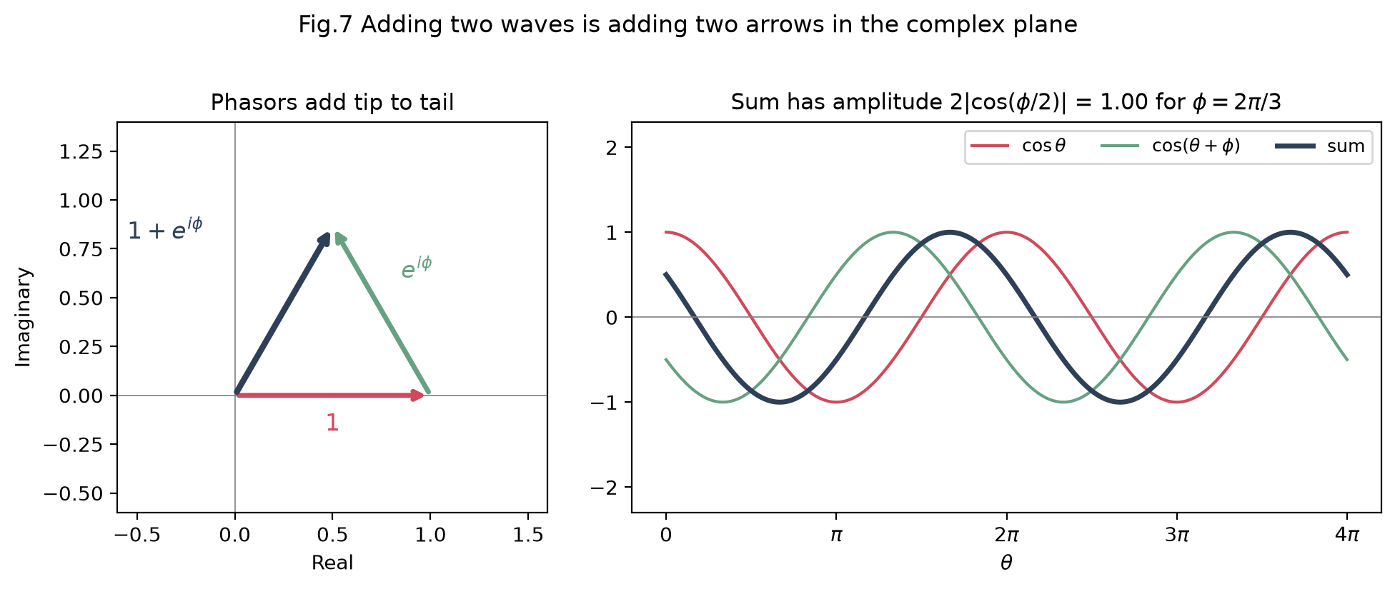

Problems¶

Problem 1: Multiplication in Cartesian form¶

Multiply $z_1 = 3 + 4i$ and $z_2 = 1 - 2i$ .

Solution

(3 + 4i)(1 - 2i) = 3 - 6i + 4i - 8i^2 = 3 - 2i + 8 = 11 - 2i.

(23)

Problem 2: Modulus¶

Find $|z|$ for $z = 7 + 24i$ .

Solution

|z| = \sqrt{7^2 + 24^2} = \sqrt{49 + 576} = \sqrt{625} = 25.

(24)

Problem 3: Division by the conjugate¶

Divide $z_1 = 3 + 4i$ by $z_2 = 1 - 2i$ .

Solution

Multiply numerator and denominator by $\bar{z}_2 = 1 + 2i$ :

\frac{(3+4i)(1+2i)}{(1-2i)(1+2i)} = \frac{-5 + 10i}{5} = -1 + 2i.

(25)

Problem 4: Multiplication in polar form¶

Multiply $z_1 = 2e^{i\pi/6}$ and $z_2 = 3e^{i\pi/3}$ .

Solution

Magnitudes multiply, angles add:

z_1 z_2 = 6\,e^{i(\pi/6 + \pi/3)} = 6\,e^{i\pi/2} = 6i.

(26)

Problem 5: Cartesian to polar¶

Express $z = -4 + 4i$ in polar form.

Solution

r = \sqrt{(-4)^2 + 4^2} = 4\sqrt{2}, \qquad \phi = \frac{3\pi}{4}\ \text{(second quadrant)},

(27)

so $z = 4\sqrt{2}\,e^{i 3\pi/4}$ .

Problem 6: Amplitude of two interfering waves¶

Show that $|1 + e^{i\phi}| = 2\left|\cos(\phi/2)\right|$ , and hence that two equal-amplitude waves with phase difference $\phi$ add to a wave of amplitude $2|\cos(\phi/2)|$ .

Solution

Factor out half the phase:

1 + e^{i\phi} = e^{i\phi/2}\left(e^{-i\phi/2} + e^{i\phi/2}\right) = 2\cos(\phi/2)\, e^{i\phi/2}.

(28)

The factor $e^{i\phi/2}$ has modulus one, so $|1 + e^{i\phi}| = 2|\cos(\phi/2)|$ . Then $\cos\theta + \cos(\theta+\phi) = \operatorname{Re}[e^{i\theta}(1+e^{i\phi})] = 2\cos(\phi/2)\cos(\theta + \phi/2)$ : a wave of the same frequency, shifted by half the phase difference, with amplitude between 0 (at $\phi = \pi$ ) and 2 (at $\phi = 0$ ).

Problem 7: A famous identity¶

Use Euler’s formula to evaluate $e^{i\pi}$ .

Problem 8: Trig from exponentials¶

Using $\cos\phi = \tfrac{1}{2}(e^{i\phi} + e^{-i\phi})$ , show that $\cos^2\phi = \tfrac{1}{2}(1 + \cos 2\phi)$ .

Problem 9: Phase rotation¶

A quantum amplitude picks up a phase, $\psi \to e^{i\theta}\psi$ . Show that the probability density $|\psi|^2$ is unchanged.

Problem 10: Derivatives of a rotating phase¶

For $u(x,t) = e^{i(kx - \omega t)}$ compute $\partial^2 u/\partial x^2$ and $\partial^2 u/\partial t^2$ , and show that $\dfrac{\partial^2 u}{\partial x^2} = \dfrac{k^2}{\omega^2}\dfrac{\partial^2 u}{\partial t^2}$ . What is the speed $v = \omega/k$ of this wave?