Fourier Transforms - Quantum Mechanics for Chemistry

Fourier Series¶

The Fourier series enables us to represent periodic functions as infinite sums. In particular, it represents a function as a sum of weighted $\sin$ and $\cos$ functions.

This is possible because the $\sin$ and $\cos$ functions form a complete orthogonal set (basis functions). The Fourier series for a function $f(x)$ with a period of $2{\pi}$ is given by:

Fourier coefficients and orthogonality of sin and cos functions

Using the orthogonality property of the $\cos$ and $\sin$ functions, we can determine an expression for the coefficients of the Fourier series. By integrating the Fourier series over the interval [- ${\pi}$ , ${\pi}$ ], we can determine an expression for $a_0$ . Over this interval the sums vanish, since we are integrating the $\sin$ and $\cos$ functions over one period. Thus, we are left with

\int_{-{\pi}}^{\pi} f(x)dx = \int_{-{\pi}}^{\pi}\frac{a_0}{2}dx.

(4)

Therefore, by carrying out the integral we find the expression for $a_0$ to be

a_0 = \frac{1}{\pi} \int_{-{\pi}}^{\pi} f(x)dx.

(5)

From this, it is clear that the $\frac{a_0}{2}$ term in the series represents the mean of the function $f(x)$ over the period. To determine the $a_n$ coefficients, we multiply the series by $\cos(mx)$ , for a positive integer $m$ , and integrate over its period. The series becomes

\int_{-{\pi}}^{\pi}f(x)\cos(mx)dx = \frac{a_0}{2}\int_{-{\pi}}^{\pi}\cos(mx)dx + \sum \limits _{n=1} ^{\infty}\int_{-{\pi}}^{\pi}a_n\cos(nx)\cos(mx)dx + \sum \limits _{n=1} ^{\infty}\int_{-{\pi}}^{\pi}b_n\sin(nx)\cos(mx)dx.

(6)

Due to the orthogonality property of the $\sin$ and $\cos$ functions, the only term that does not vanish on the right-hand side is $\int_{-{\pi}}^{\pi}a_n\cos(nx)\cos(mx)dx$ for $m=n$ . Solving for $a_n$ we get

a_n = \frac{1}{\pi} \int_{-{\pi}}^{\pi} f(x)\cos(nx)dx \,\,\,\,n=1, 2, ...

(7)

This is consistent with the expression for $a_0$ when $n=0$ . Thus the factor of 1/2 included on the $a_0$ term is there to maintain this consistency between $a_0$ and $a_n$ .
To determine the values of the $b_n$ coefficients, we multiply by $\sin(mx)$ . As with the $a_n$ coefficients, by the orthogonality property the only term that does not vanish on the right-hand side is $\int_{-{\pi}}^{\pi}b_n\sin(nx)\sin(mx)dx$ for $m=n$ . Thus, solving for $b_n$ ,

b_n = \frac{1}{\pi} \int_{-{\pi}}^{\pi} f(x)\sin(nx)dx \,\,\,\,n=1, 2, ...

(8)

Square function and Gibbs phenomenon¶

Now that we have introduced the Fourier series, let’s look at an example: the positive square wave. This is defined as

f(x) = \left\{ \begin{array}{ll} 0 & \text{if } -\pi \leq x < 0, \\ 1 & \text{if } 0 \leq x < \pi, \\ \end{array} \right.

(9)

Let’s plot this function.

# Define a function to create a square wave
import numpy as np
import matplotlib.pyplot as plt

def square(x, period):
    # Create array with zeros
    y = np.zeros(len(x))
    # Change zeros to 1 based on a given period in radians (e.g. 2pi, 3pi)
    for i in range(len(x)):
        if (x[i] / period) % 1 < 0.50:
            y[i] = 1.0
    return y

N = 1000  # Number of points
x = np.linspace(-10.0, 10.0, N)

plt.figure(figsize=(7, 4))
plt.plot(x, square(x, 2 * np.pi))
plt.grid(True)
plt.ylim(-0.2, 1.2)
plt.xlabel('x')
plt.show()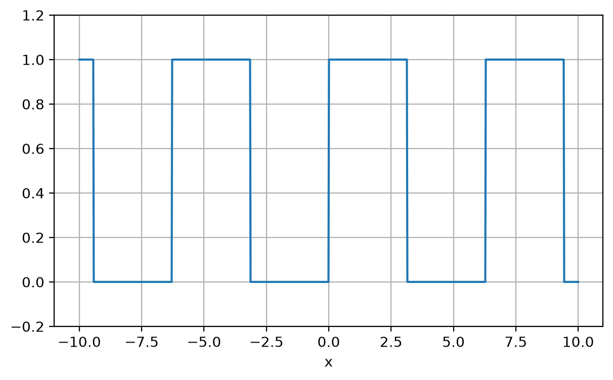

Now let’s try to express the square wave as a Fourier series. First, we calculate the coefficients using the expressions above. Carrying out the calculations, we find

a_0 = \frac{1}{\pi} \int_{0}^{\pi} dx = 1,\\ a_n = \frac{1}{\pi} \int_{0}^{\pi} \cos(nx)dx = 0, \,\,\,\,n\geq 1,

(10)

b_n = \frac{1}{\pi} \int_{0}^{\pi} \sin(nx)\,dx = \left\{ \begin{array}{ll} \frac{2}{n\pi} & \text{if } n \text{ is odd}, \\ 0 & \text{if } n \text{ is even}. \\ \end{array} \right.

(11)

Now let’s plot the Fourier series for $n=10, n=50,$ and $n=100$ .

# Define the cos and sin terms of the Fourier series
def cosTerm(n):
    # Always zero except for n=0
    if n==0: return 1.0
    return 0.

def sinTerm(n):

    if n%2: # n modulo 2 = 1 (True) then Odd
        ret = 2. / (n* np.pi)
    else:
        ret = 0.
    return ret

def fourier(n,x):
    #a_0 term, remember 1/2
    sum = cosTerm(0)/2.0 * np.ones(len(x))
    
    #all other terms
    for i in range(1, n+1):
        sum += sinTerm(i)*np.sin(i*x) + cosTerm(i)*np.cos(i*x)
    return sum

fig, axes = plt.subplots(1, 3, figsize=(14,4), sharey=True)

# Loop over each subplot
for idx, i in enumerate([10, 50, 100]):
    ax = axes[idx]
    ax.plot(x, fourier(i, x), label="n = %g" % (i))
    ax.plot(x, square(x, 2*np.pi), color="black", label="square wave")
    ax.legend(loc="upper right", fontsize="small")
    ax.set_xlabel("x")
    ax.set_ylim(-0.2, 1.2)
    
plt.tight_layout()
plt.show()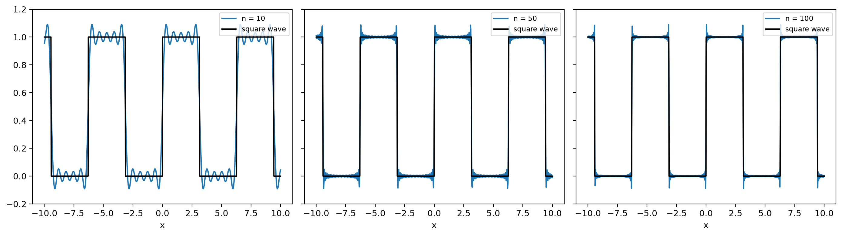

Fourier Transform¶

Recall that Euler’s formula expresses $e^{ix}$ in terms of sines and cosines, so we can also write the Fourier series using complex numbers:

f(x)=\sum_{n=0}^{\infty} c_{n} \exp \left(i \frac{2 \pi n x}{L}\right)

(12)

And the coefficients would then be:

c_{n}=\frac{1}{L} \int_{-\frac{L}{2}}^{\frac{L}{2}} f(x) \exp \left(-i \frac{2 \pi n x}{L}\right) d x

(13)

We might not like the use of complex numbers, but it is clearly the same Fourier series. We can also simplify the notation a bit by introducing the “wave number”

k_{n}=\frac{2 \pi n}{L} = \frac{2 \pi}{\lambda}

(14)

where $\lambda$ is the wavelength. If we let the length $L$ go to infinity, then:

\Delta k_{n}=\frac{2 \pi n}{L} \rightarrow d k

(15)

the coefficients are:

c(k)=\frac{1}{2 \pi} \int_{-\infty}^{\infty} f(x) \mathrm{e}^{-i k x} d x

(16)

Fourier analysis of time-series data¶

Periodic data¶

We’re going to construct an array of time points. Then we’ll set up a function with two sine waves:

y = \sin(30 \cdot 2\pi t) + \frac{1}{2} \sin(50 \cdot 2 \pi t)

(19)

We can use scipy.fftpack to perform the “fast Fourier transform” (FFT). The resulting “x” variable is in frequency, so its limit is set by the $dt$ we used. We cannot find a frequency higher than that time resolution allows. (In short, if we expected GHz signals, we would need a short time resolution.)

import scipy.fftpack

# Number of sample points
N = 1000
# Sample spacing
delta = 1.0 / 1000.0

# Time array
t = np.linspace(0.0, delta * N, N)

# Time domain signal
y = np.sin(30.0 * 2.0 * np.pi * t) + 0.5 * np.sin(50.0 * 2.0 * np.pi * t)

# Compute the Fourier Transform
xf = np.linspace(0.0, 1.0 / (2.0 * delta), N // 2)
yf = scipy.fftpack.fft(y)

# Plot both time domain and frequency domain side by side
fig, (ax1, ax2) = plt.subplots(1, 2, figsize=(12, 6))

# Time domain plot
ax1.plot(t, y)
ax1.set_xlabel("Time")
ax1.set_ylabel("Amplitude")
ax1.set_title("Time Domain Signal")

# Frequency domain plot
ax2.plot(xf, 2.0 / N * np.abs(yf[:N // 2]))
ax2.set_xlabel("Frequency")
ax2.set_ylabel("Amplitude")
ax2.set_title("Frequency Domain Signal")

plt.tight_layout()
plt.show()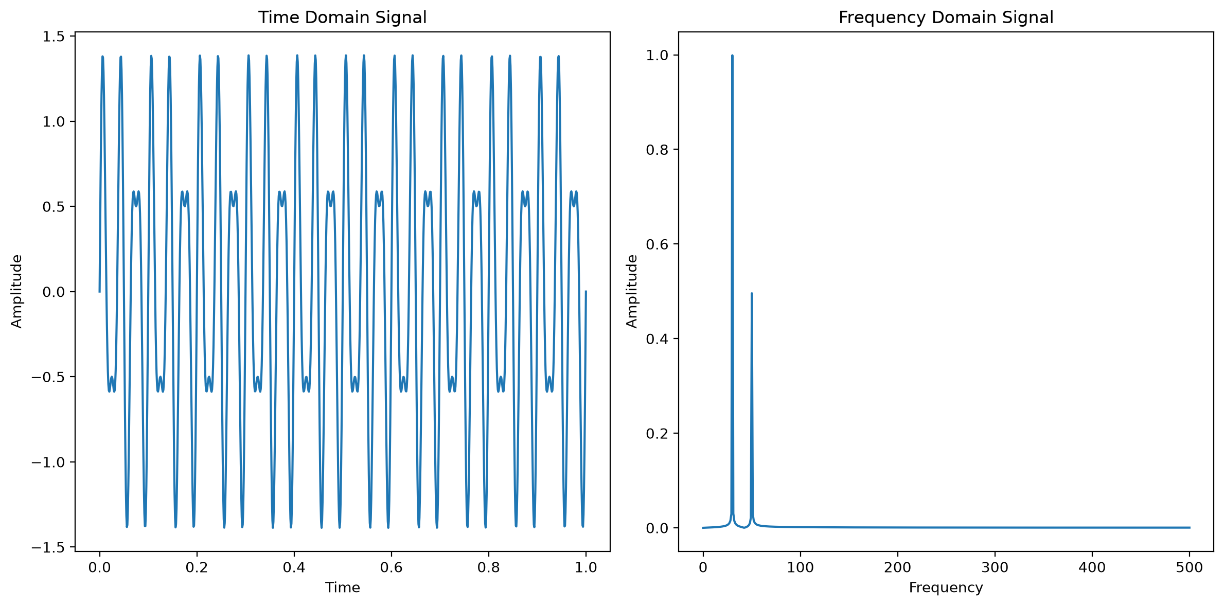

Notice that it is not a perfect reconstruction. We only put in two specific frequencies, so we would expect to see two sharp lines. But if the waves are not exactly periodic when we cut off the time signal, the peaks acquire a bit of width.
The time-domain signal can be as complicated as we want. Here is an example with four frequencies. Note that the phase, whether indicated by a sine or a cosine function, does not matter: both are periodic.

Noisy periodic data¶

import numpy as np
import matplotlib.pyplot as plt
from scipy.fftpack import fft

# Generate sample data
t = np.linspace(0.0, 1.0, 500)
y = np.sin(30.0 * 2.0 * np.pi * t) + 0.5 * np.cos(50.0 * 2.0 * np.pi * t)
y = y + 1.5 * np.sin(165.0 * 2.0 * np.pi * t) + np.cos(104 * 2.0 * np.pi * t)

# Compute the Fourier Transform
N = len(t)
yf = fft(y)
xf = np.fft.fftfreq(N, t[1] - t[0])[:N//2]

# Plot both time domain and frequency domain side by side
fig, (ax1, ax2) = plt.subplots(1, 2, figsize=(12, 6))

# Time domain plot
ax1.plot(t, y)
ax1.set_xlabel("Time")
ax1.set_ylabel("Amplitude")
ax1.set_title("Time Domain Signal")

# Frequency domain plot
ax2.plot(xf, 2.0 / N * np.abs(yf[:N//2]))
ax2.set_xlabel("Frequency")
ax2.set_ylabel("Amplitude")
ax2.set_title("Frequency Domain Signal")

# Show the plots
plt.tight_layout()
plt.show()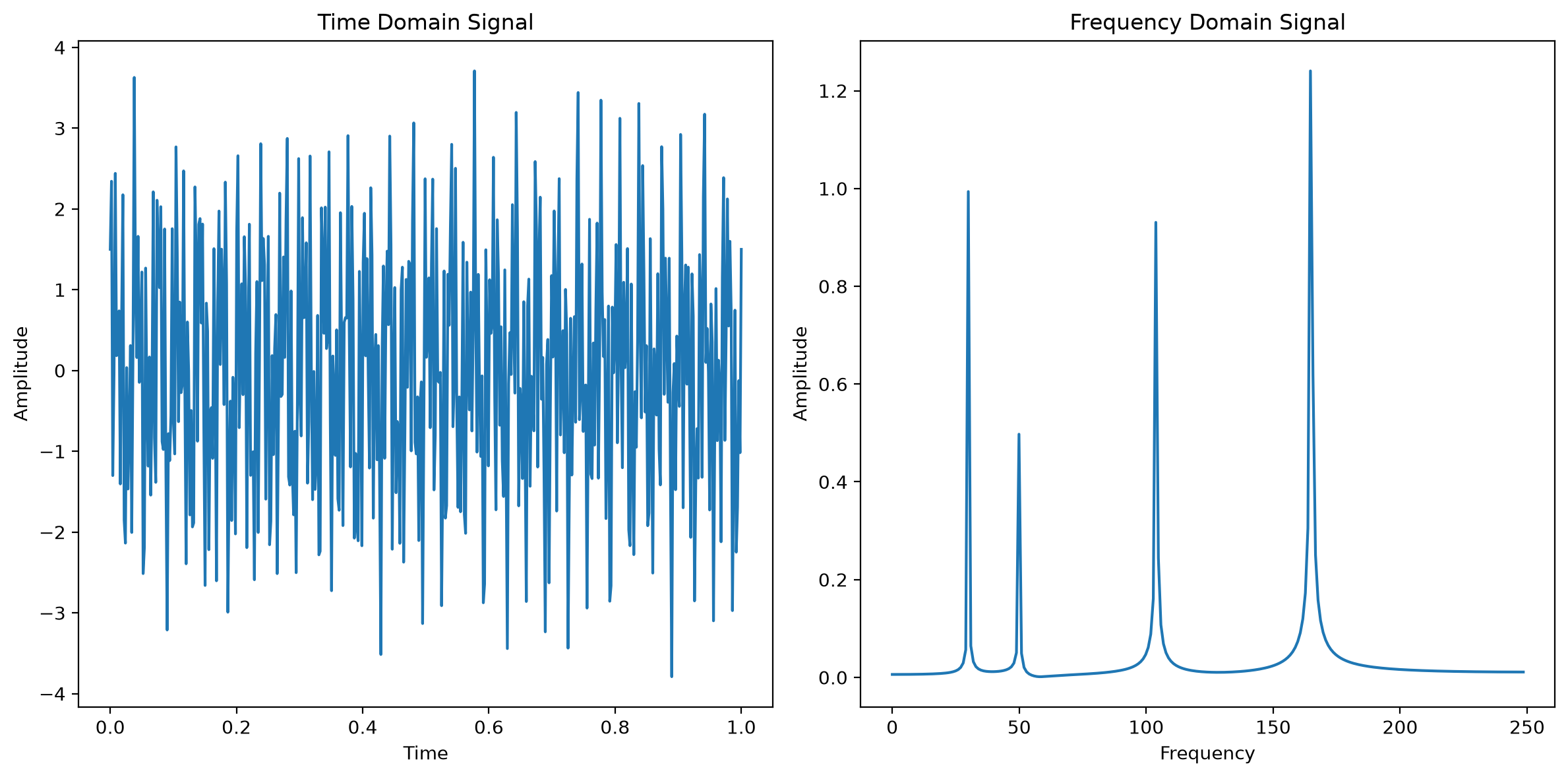

Noisy non-periodic data¶

Whatever signals we put into our time function will come out of the FFT, at least within the time resolution we start with. (We cannot find 800 Hz frequencies in this example.)
Also, the time signal need not be completely periodic. A “chirp,” where the signal intensity drops over time, also works.

# Apply the exponential decay to the time domain signal
y = y * np.exp(-2 * t)

# Compute the Fourier Transform after the decay
yf = fft(y)

# Plot both time domain and frequency domain side by side
fig, (ax1, ax2) = plt.subplots(1, 2, figsize=(12, 6))

# Time domain plot after exponential decay
ax1.plot(t, y)
ax1.set_xlabel("Time")
ax1.set_ylabel("Amplitude")
ax1.set_title("Time Domain Signal with Exponential Decay")

# Frequency domain plot after exponential decay
ax2.plot(xf, 2.0 / N * np.abs(yf[:N//2]))
ax2.set_xlabel("Frequency")
ax2.set_ylabel("Amplitude")
ax2.set_title("Frequency Domain Signal with Exponential Decay")

# Show the plots
plt.tight_layout()
plt.show()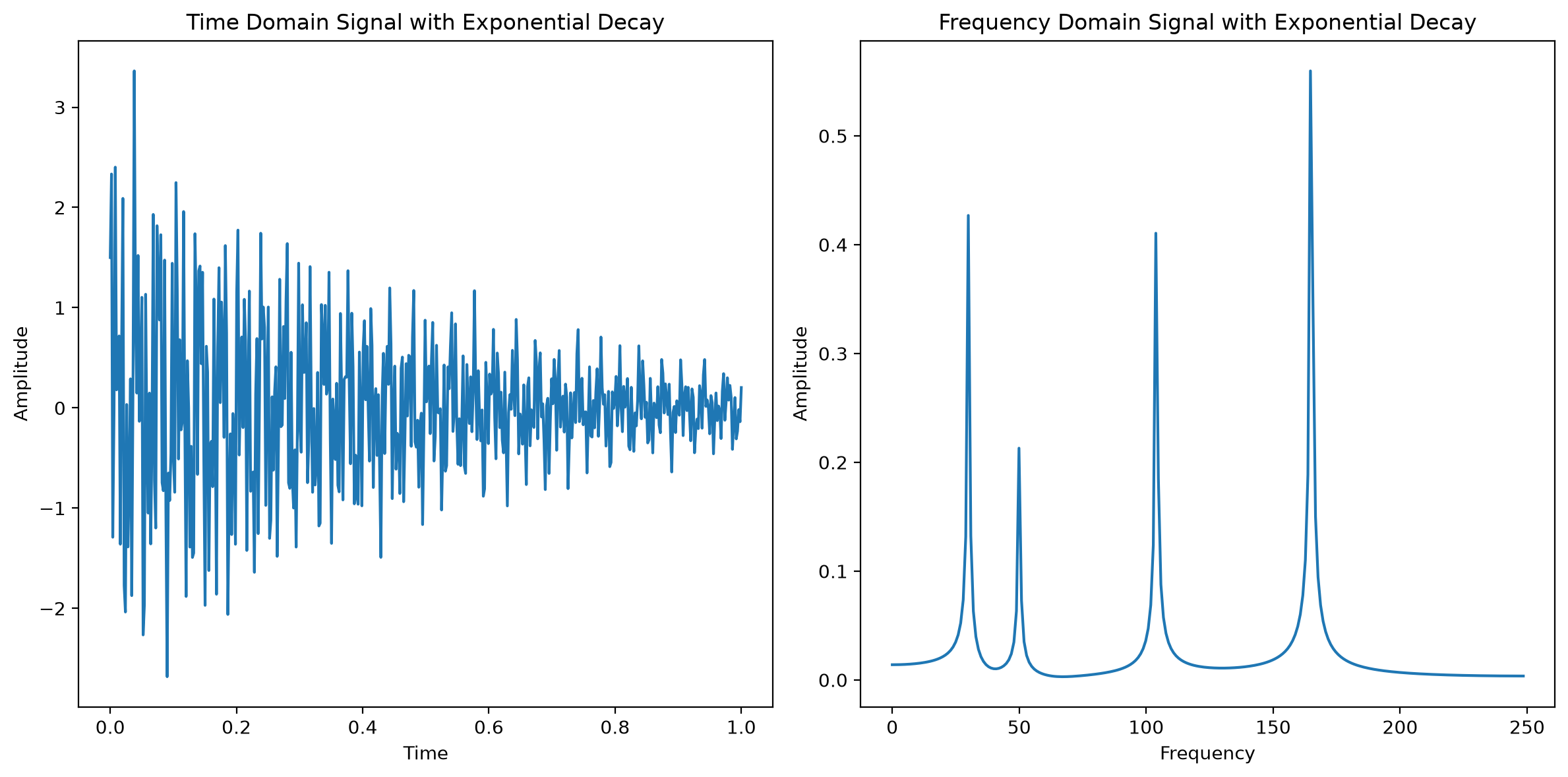

Notice that while the peak heights changed a bit, the relative intensities and peak areas remain unchanged. So if you are doing spectroscopy, you need a few wave repeats, but it need not be a “continuous wave” spectrum. This is useful if you are worried about applying a high-intensity beam (e.g. an x-ray).

Fourier transform and the uncertainty relation¶

Define the Square Function to represent $\psi(x)$ : Start with a square function (or rectangular pulse) that has a width $w$ and height 1, centered around zero. This function can be represented as:

\psi(x) = \begin{cases} 1, & |x| \leq \frac{w}{2} \\ 0, & |x| > \frac{w}{2} \end{cases}

(20)

Fourier Transform gives us $\psi(p)$ : The Fourier transform $\hat{f}(k)$ of a square function is a sinc function:

\hat{\psi}(k) = w \, \text{sinc}(kw/2)

(21)

where $\text{sinc}(x) = \frac{\sin(x)}{x}$ . This shows how the Fourier transform spreads out as the width of the square function changes.

The uncertainty principle states that the product of the standard deviations of a function and its Fourier transform is bounded by a minimum value!
Here, $\Delta x$ is the width of the function (related to the spread in position), and $\Delta k$ is the spread of the Fourier transform (momentum space). As the width $w$ of the square function decreases, the spread of the sinc function in the Fourier domain increases, demonstrating the uncertainty relation.
In quantum mechanics, using the de Broglie relation, we can recover the uncertainty relation since $k=2\pi/\lambda = 2\pi p/h = p/\hbar$ .

import matplotlib.pyplot as plt
from matplotlib.animation import FuncAnimation
from IPython.display import HTML
import numpy as np

# Define the square function
def square_function(x, w):
    return np.where(np.abs(x) <= w / 2, 1, 0)

# Fourier transform of the square function (sinc function)
def fourier_transform_square_function(k, w):
    return w * np.sinc(k * w / (2 * np.pi))

# Define x and k ranges
x = np.linspace(-5, 5, 1000)
k = np.linspace(-20, 20, 1000)

# Set up the figure and axes for animation
fig, axes = plt.subplots(2, 1, figsize=(8, 8))

# Initialize the plots
line1, = axes[0].plot([], [], lw=2)
axes[0].set_ylim([-0.1, 1.1])
axes[0].set_title("Square Function")

line2, = axes[1].plot([], [], lw=2)
axes[1].set_ylim([-0.5, 2.5])
axes[1].set_title("Fourier Transform")

# Set the x-axis limits
axes[0].set_xlim(x.min(), x.max())
axes[1].set_xlim(k.min(), k.max())

# Initialization function
def init():
    line1.set_data([], [])
    line2.set_data([], [])
    return line1, line2

# Animation update function
def update(w):
    # Compute the square function and its Fourier transform
    sq_func = square_function(x, w)
    ft_sq_func = fourier_transform_square_function(k, w)
    
    # Update the data for both plots
    line1.set_data(x, sq_func)
    line2.set_data(k, ft_sq_func)
    
    return line1, line2

# Create the animation
ani = FuncAnimation(fig, update, frames=np.linspace(0.1, 5.0, 100), init_func=init, blit=True)

plt.close(fig)  # Prevents static display of the last frame
HTML(ani.to_jshtml())

Fourier transforms of Gaussian functions¶

A Gaussian function is defined as

f(t) = \exp\left(- \frac{t^2}{2{\sigma^2}}\right),

(23)

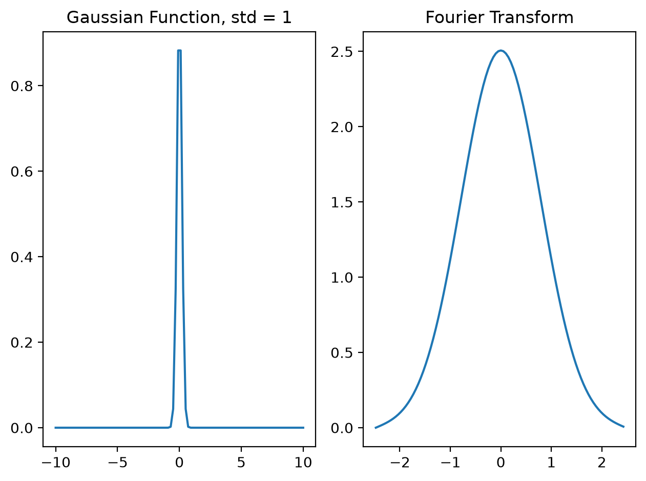
where $\sigma$ is the standard deviation of the Gaussian. The Fourier transform of a Gaussian is another Gaussian, such that

\mathcal{F}[f(t)] = \sqrt{2\pi}\, \exp\left(- \frac{\omega^2\sigma^2}{2}\right)

(24)

Thus we can see that as the Gaussian function gets broader, its Fourier transform gets narrower. To illustrate this, let’s plot the Gaussian and its transform for two different standard deviations.

from scipy import signal

g1 = signal.windows.gaussian(100, std=10)
t = np.linspace(-10, 10, len(g1))

plt.subplot(1, 2, 1)
plt.plot(t, g1)
plt.title('Gaussian Function, std = 10')

FT_omega = np.fft.fftfreq(len(g1), t[1] - t[0])
FT = np.fft.fft(g1)
FT_omega = np.fft.fftshift(FT_omega)
FT = np.fft.fftshift(FT)

plt.subplot(1, 2, 2)
plt.plot(FT_omega, abs(FT))
plt.title('Fourier Transform')
plt.tight_layout()
plt.show()

g2 = signal.windows.gaussian(100, std=1)
t = np.linspace(-10, 10, len(g2))

plt.subplot(1, 2, 1)
plt.plot(t, g2)
plt.title('Gaussian Function, std = 1')

FT_omega = np.fft.fftfreq(len(g2), t[1] - t[0])
FT = np.fft.fft(g2)
FT_omega = np.fft.fftshift(FT_omega)
FT = np.fft.fftshift(FT)

plt.subplot(1, 2, 2)
plt.plot(FT_omega, abs(FT))
plt.title('Fourier Transform')
plt.tight_layout()
plt.show()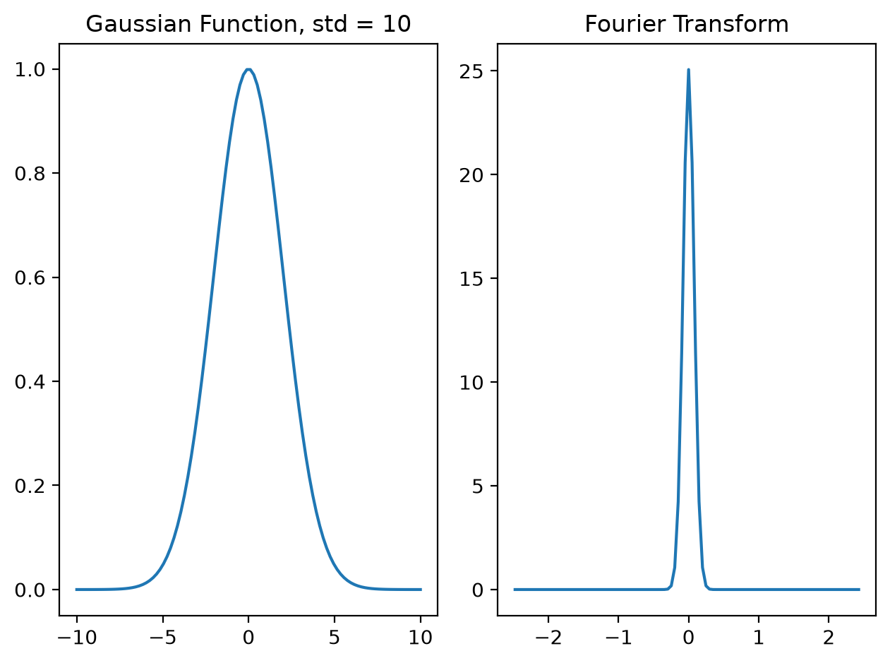

Delta Function¶

The delta function, $\delta(t)$ , is defined as

\delta(t) = \left\{ \begin{array}{ll} 0 & \text{if } t \neq 0, \\ \infty & \text{if } t = 0. \end{array} \right.

(25)

Carrying out the transform, we see that the Fourier transform of the delta function is actually a constant, such that

\mathcal{F}[{\delta}(t)] = 1

(26)

Let’s plot the function and its transform.

from scipy import signal
imp = signal.unit_impulse(100, 'mid') # creates the delta function
t = np.linspace(-5, 5, 100)

plt.subplot(1,2,1)
plt.plot(t, imp)
plt.title('Delta Function')

FT_omega = np.fft.fftfreq(100, t[1] - t[0])
FT = np.fft.fft(imp)

plt.subplot(1,2,2)
plt.plot(FT_omega, abs(FT))
plt.title('Fourier Transform')
plt.ylim([0,1.2])
plt.tight_layout()
plt.show()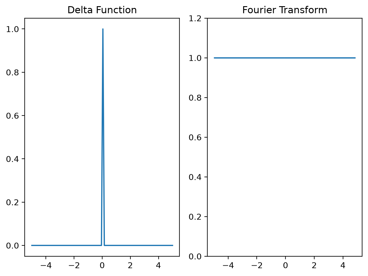

Free Electron and Delta Function Duality¶

A general wavefunction can be expanded as a superposition of momentum eigenstates:

\psi(x) = \frac{1}{\sqrt{2\pi}} \int \phi(k)\, e^{ikx}\, dk,

(27)

where $e^{ikx}$ are eigenfunctions of the free-particle Hamiltonian and form a complete orthogonal basis. The coefficient $\phi(k)$ gives the amplitude of each momentum mode.

For a localized particle, $\phi(k)$ is broad: many momenta combine to form a narrow spatial peak.
For a free electron with definite momentum $k_0$ ,
$\phi(k) = \delta(k - k_0),$
(28)
so that
$\psi(x) = e^{ik_0x}.$
(29)
- Conversely, for a localized particle at $x_0$ :
$\psi(x) = \delta(x - x_0) \;\Rightarrow\; \phi(k) = \frac{1}{\sqrt{2\pi}} e^{-ikx_0}.$
(30)
Thus, a free electron (plane wave) is a single momentum component spread uniformly in space, while a localized delta function in space is an infinite superposition of plane waves. This Fourier duality expresses the position-momentum uncertainty relationship.