Under the calculus of quantum mechanics lies a simpler and more powerful truth: it is all linear algebra. Wavefunctions are vectors, operators are matrices, and the Schrodinger equation is the eigenvalue problem in disguise. This appendix makes that correspondence concrete and visual. It does not re-derive the differential equations of the course: separation of variables, the wave equation, and their oscillating and decaying solutions are developed in detail in Chapter 2 on waves. Here we stay on the linear-algebra side and show how operators become matrices you can build, picture, and diagonalize.
Functions are vectors, operators are matrices
A function is a vector with one component per point
Take any function and evaluate it at points . The list of values is a vector with components. For example sampled at becomes the vector .
Now let the grid get finer, with spacing . The vector gains a component for every point , and in that limit the function is an infinite-dimensional vector. The value plays the role of “the component at ,” exactly as is the component of along basis direction . The left panel below shows a smooth function and the vector of samples that stands in for it on a grid.
Source
import numpy as np
import matplotlib.pyplot as plt

fig, axes = plt.subplots(1, 2, figsize=(10, 3.6))

# Panel a: sampling a function on a grid
xf = np.linspace(0, 2 * np.pi, 300)
xg = np.linspace(0, 2 * np.pi, 13)
axes[0].plot(xf, np.sin(xf), 'k', lw=1.5, label=r'$f(x)=\sin x$')
axes[0].vlines(xg, 0, np.sin(xg), color='#d1495b', lw=0.8)
axes[0].plot(xg, np.sin(xg), 'o', color='#d1495b', ms=6, label='samples = vector components')
axes[0].axhline(0, color='gray', lw=0.6)
axes[0].set_xlabel('x')
axes[0].legend(fontsize=8, loc='upper right')
axes[0].set_title('Fig.1a A function becomes a vector of samples')

# Panel b: the three-point second-derivative stencil
pts = np.arange(7)
axes[1].plot(pts, np.zeros_like(pts), 'o', color='0.8', ms=13)
for p, w, c in [(2, '+1', '#d1495b'), (3, '-2', '#2e4057'), (4, '+1', '#d1495b')]:
    axes[1].plot(p, 0, 'o', color=c, ms=15)
    axes[1].text(p, 0.18, w, ha='center', color=c, fontsize=12, fontweight='bold')
axes[1].annotate('point j', xy=(3, 0), xytext=(3, -0.35), ha='center',
                 color='#2e4057', fontsize=10)
axes[1].set_ylim(-0.6, 0.6)
axes[1].set_xlim(-0.5, 6.5)
axes[1].axis('off')
axes[1].set_title(r'Fig.1b The stencil $(1,-2,1)$ for $d^2/dx^2$ at point j')

plt.tight_layout()
plt.show()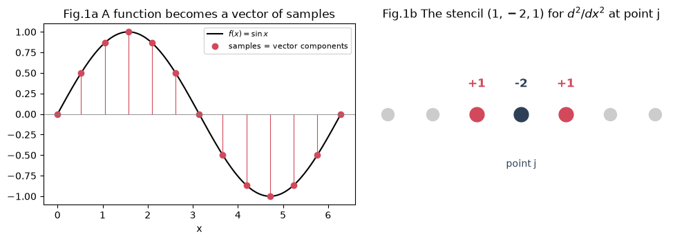
The inner product becomes an integral
This is the link that makes the analogy precise. The dot product of two vectors sums the products of matching components. For function-vectors, that sum over grid points, weighted by the spacing , is a Riemann sum, and in the fine-grid limit it becomes an integral:
So the quantum-mechanical inner product is nothing more than the dot product from the previous page, carried to infinite dimensions. Everything built on the dot product carries over verbatim: normalization is just , and orthogonal wavefunctions () are just perpendicular vectors.
An operator is a matrix
A linear operator takes a function and returns a function, that is, it takes a vector and returns a vector. Any linear map on vectors is a matrix, so every quantum operator is a matrix acting on the function-vector. This gives the full dictionary between the linear algebra you already know and the quantum mechanics ahead:
| Linear algebra (finite dimensions) | Quantum mechanics (functions) |
|---|---|
| vector | wavefunction |
| component | value |
| dot product | inner product |
| normalized | normalized |
| orthonormal basis | orthonormal functions |
| matrix | operator (such as , , ) |
| eigenvector equation | eigenfunction equation |
| eigenvalue | measured value (energy, momentum) |
| Hermitian matrix | Hermitian operator (real eigenvalues) |
| unitary matrix | time evolution, symmetry operations |
| expansion | superposition |
The derivative as a matrix: the stencil
The recipe for turning a derivative into a matrix is the stencil: a small pattern of weights applied to each grid point and its neighbors. The first derivative uses a centered difference, the slope between the neighbor on the left and the neighbor on the right:
Written as a matrix acting on the sampled vector (with one-sided formulas at the two boundaries), this is
import numpy as np

n = 5
x = np.linspace(0, 4, n)
dx = x[1] - x[0]
psi = x**2

D1 = (1 / (2 * dx)) * np.array([
    [-3, 4, -1, 0, 0],
    [-1, 0, 1, 0, 0],
    [0, -1, 0, 1, 0],
    [0, 0, -1, 0, 1],
    [0, 0, 1, -4, 3],
])

print("finite-difference derivative of x^2:", D1 @ psi)
print("exact derivative 2x               :", 2 * x)
finite-difference derivative of x^2: [0. 2. 4. 6. 8.]
exact derivative 2x : [0. 2. 4. 6. 8.]
The second derivative uses the three-point stencil over , the pattern sketched in Fig.1b. Because each point couples only to its two neighbors, the matrix is banded (tridiagonal): almost all entries are zero. The left panel below shows that sparsity pattern; the right panel confirms the matrix works by turning into , since .
Source
import numpy as np
import matplotlib.pyplot as plt

N = 200
x = np.linspace(0, 2 * np.pi, N)
dx = x[1] - x[0]

# Second-derivative matrix, tridiagonal (1, -2, 1) / dx^2
D2 = (np.diag(np.ones(N - 1), 1)
      - 2 * np.diag(np.ones(N))
      + np.diag(np.ones(N - 1), -1)) / dx**2

fig, axes = plt.subplots(1, 2, figsize=(10, 3.8))

# Panel a: sparsity pattern of a small D2 (banded / tridiagonal)
small = (np.diag(np.ones(11), 1) - 2 * np.diag(np.ones(12)) + np.diag(np.ones(11), -1))
axes[0].spy(small, markersize=8, color='#2e4057')
axes[0].set_title('Fig.2a $D_2$ is banded: each point couples to neighbors')
axes[0].set_xlabel('column'); axes[0].set_ylabel('row')

# Panel b: apply D2 to sin x
psi = np.sin(x)
d2psi = D2 @ psi
axes[1].plot(x, psi, 'k', lw=2, label=r'$\psi = \sin x$')
axes[1].plot(x[1:-1], d2psi[1:-1], color='#d1495b', lw=2, label=r'$D_2\,\psi$')
axes[1].plot(x, -np.sin(x), '--', color='#66a182', lw=2, label=r'$-\sin x$ (exact)')
axes[1].axhline(0, color='gray', lw=0.6)
axes[1].set_xlabel('x')
axes[1].legend(fontsize=9, loc='upper right')
axes[1].set_title('Fig.2b The matrix turns sin x into -sin x')

plt.tight_layout()
plt.show()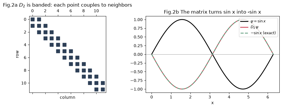
Diagonalizing this second-derivative matrix (plus a potential on the diagonal) is exactly how a computer finds energies and wavefunctions. That is the whole idea behind the numerical Schrodinger solver.
From 1D to 2D grids
Nothing about the stencil idea is special to one dimension. On a 2D grid, the natural second-derivative operator is the Laplacian , whose continuous meaning is explored in div, grad, curl. Discretized, it becomes the five-point stencil: the center point with weight -4 and its four nearest neighbors with weight +1.
To store a 2D grid of values as a single vector, we flatten it row by row. The Laplacian is then still a matrix, now with a block-banded sparsity pattern: the horizontal neighbors sit on the near diagonals, and the vertical neighbors appear as off-diagonal blocks one grid-row away.
Source
import numpy as np
import matplotlib.pyplot as plt

fig, axes = plt.subplots(1, 2, figsize=(10, 4.2))

# Panel a: 2D grid with the five-point stencil highlighted
m = 5
for i in range(m):
    for j in range(m):
        axes[0].plot(i, j, 'o', color='0.82', ms=13)
cx, cy = 2, 2
for dx, dy in [(1, 0), (-1, 0), (0, 1), (0, -1)]:
    axes[0].annotate('', xy=(cx + dx, cy + dy), xytext=(cx, cy),
                     arrowprops=dict(arrowstyle='->', color='#d1495b', lw=1.5))
    axes[0].plot(cx + dx, cy + dy, 'o', color='#d1495b', ms=15)
    axes[0].text(cx + dx, cy + dy + 0.22, '+1', ha='center', color='#d1495b', fontsize=10)
axes[0].plot(cx, cy, 'o', color='#2e4057', ms=17)
axes[0].text(cx, cy + 0.24, '-4', ha='center', color='white', fontsize=9, fontweight='bold')
axes[0].set_xlim(-0.6, 4.6); axes[0].set_ylim(-0.6, 4.6)
axes[0].set_aspect('equal'); axes[0].axis('off')
axes[0].set_title('Fig.3a The five-point Laplacian stencil')

# Panel b: sparsity of the 2D Laplacian, built by a Kronecker sum
n = 6
lap1d = -2 * np.eye(n) + np.eye(n, k=1) + np.eye(n, k=-1)
eye = np.eye(n)
lap2d = np.kron(lap1d, eye) + np.kron(eye, lap1d)   # (n^2) x (n^2)
axes[1].spy(lap2d, markersize=4, color='#2e4057')
axes[1].set_title(f'Fig.3b 2D Laplacian on a {n}x{n} grid ({n*n}x{n*n} matrix)')
axes[1].set_xlabel('column'); axes[1].set_ylabel('row')

plt.tight_layout()
plt.show()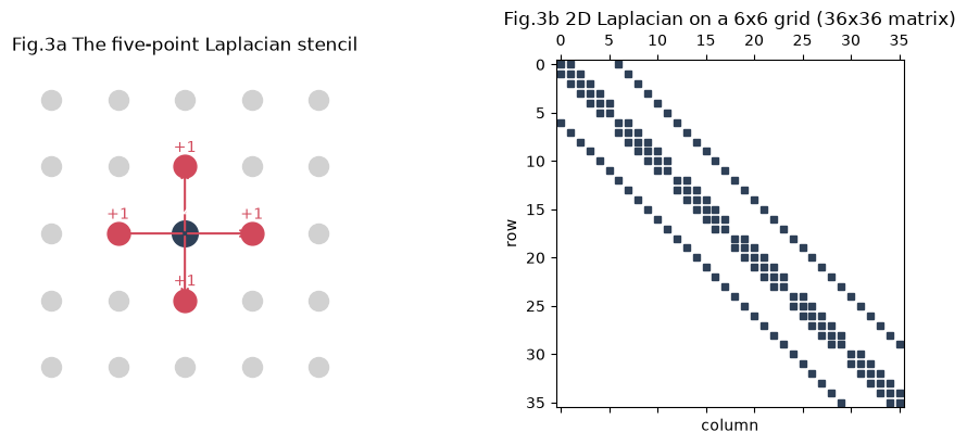
The np.kron (Kronecker product) construction is the standard way to assemble multidimensional operators from 1D pieces: . The same trick builds 3D operators for real atoms and molecules. The matrix grows fast ( for an grid), but it stays overwhelmingly sparse, which is what makes large quantum calculations feasible.
Matrices are linear operators
Acting with a matrix is a linear operation: it respects sums and scalar multiples,
This is the same linearity that defines a quantum operator, which is why a matrix and an operator are the same kind of object. One consequence is immediate and important: order matters. Matrices generally do not commute, .
import numpy as np

A = np.array([[1, 2], [0, 1]])   # a shear
B = np.array([[0, 1], [1, 0]])   # a swap

print("AB =\n", A @ B)
print("BA =\n", B @ A)
print("\ncommutator AB - BA =\n", A @ B - B @ A)
AB =
[[2 1]
[1 0]]
BA =
[[0 1]
[1 2]]
commutator AB - BA =
[[ 2 0]
[ 0 -2]]
Applying a shear then a swap is not the same as a swap then a shear. In quantum mechanics this non-commutation, packaged as the commutator , is exactly what forbids simultaneous sharp values of position and momentum. It is the algebra behind the uncertainty principle.
The two special matrices of quantum mechanics
Out of all matrices, quantum mechanics leans on just two families, distinguished by how they relate to their conjugate transpose (transpose, then complex-conjugate each entry).
Hermitian matrices: real eigenvalues
Because measured values are real, every observable (energy, position, momentum) is represented by a Hermitian operator. The reality of the eigenvalues is what guarantees a measurement returns a real number, and the orthogonality of eigenvectors is why distinct energy levels give orthogonal stationary states.
import numpy as np

# A Hermitian matrix: A^dagger = A (note the i and -i off the diagonal)
A = np.array([[2.0, 1.0 - 1j],
              [1.0 + 1j, 3.0]])
print("Hermitian? A == A^dagger:", np.allclose(A, A.conj().T))

vals, vecs = np.linalg.eigh(A)
print("eigenvalues (all real):", vals)
# eigenvectors orthonormal: V^dagger V = I
print("eigenvectors orthonormal:", np.allclose(vecs.conj().T @ vecs, np.eye(2)))
Hermitian? A == A^dagger: True
eigenvalues (all real): [1. 4.]
eigenvectors orthonormal: True
Unitary matrices: they preserve length
Because probability is the squared norm of the wavefunction, anything that must conserve probability is unitary: time evolution and symmetry operations are all unitary. They rotate the state vector without changing its length.
Source
import numpy as np
import matplotlib.pyplot as plt

theta = 0.7
U = np.array([[np.cos(theta), -np.sin(theta)],
              [np.sin(theta),  np.cos(theta)]])   # a rotation: real unitary

v = np.array([3.0, 4.0])
print("U preserves length:", np.linalg.norm(U @ v), "vs", np.linalg.norm(v))
print("U^dagger U = I:", np.allclose(U.conj().T @ U, np.eye(2)))

# Eigenvalues lie on the unit circle
eigvals = np.linalg.eigvals(U)
fig, ax = plt.subplots(figsize=(4.2, 4.2))
circle = np.exp(1j * np.linspace(0, 2 * np.pi, 200))
ax.plot(circle.real, circle.imag, 'k', lw=1)
ax.plot(eigvals.real, eigvals.imag, 'o', color='#d1495b', ms=10)
ax.axhline(0, color='gray', lw=0.5); ax.axvline(0, color='gray', lw=0.5)
ax.set_aspect('equal')
ax.set_xlabel('real'); ax.set_ylabel('imaginary')
ax.set_title('Fig.4 Unitary eigenvalues sit on the unit circle')
plt.tight_layout()
plt.show()
U preserves length: 5.0 vs 5.0
U^dagger U = I: True
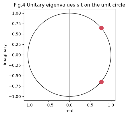
Hermitian and unitary matrices are two sides of one coin: if is Hermitian, then is unitary. Real observables generate probability-conserving evolution. That single sentence is the linear-algebra backbone of the whole theory.
Problems
Problem 1: Read off a derivative matrix
Using the first-derivative matrix above with , apply it to the constant vector . What do you expect, and why?
Solution
Each interior row computes a difference of equal neighbors, so the derivative is 0 everywhere. The derivative of a constant is zero, and the boundary rows are built to return zero for a constant as well.
Problem 2: Build a second-derivative matrix
Modify the code to build on a grid of points over , apply it to , and check that you recover .
Problem 3: A commutator
Compute the commutator for and .
Solution
Problem 4: Is it Hermitian?
Decide whether is Hermitian, and predict whether its eigenvalues are real.
Solution
The conjugate transpose swaps the off-diagonal entries and conjugates them: moves to the lower-left, which already holds . So : the matrix is Hermitian, and its eigenvalues must be real.
Problem 5: Unitary preserves length
Verify by hand that the rotation matrix satisfies , so it preserves the norm of any vector.
Problem 6: Sparsity counting
An 2D grid gives a Laplacian matrix of size . Using the five-point stencil, roughly how many nonzero entries does each row have, and why does the matrix stay sparse as grows?
Solution
Each grid point couples to itself and its four neighbors, so every row has about five nonzero entries regardless of . The matrix has rows but only about nonzeros out of possible, so the fraction filled, about , shrinks as the grid grows. This sparsity is what makes large numerical quantum calculations possible.
Problem 7: Hermitian generates unitary
Explain in one or two sentences why, if is Hermitian, the time-evolution operator is unitary and therefore conserves probability.