Bead, spring and a wall
The classical harmonic oscillator is a system of a bead attached to a wall with a spring.
When the bead is displaced from its equilibrium or resting position to some point , it experiences a restoring force proportional to the displacement :
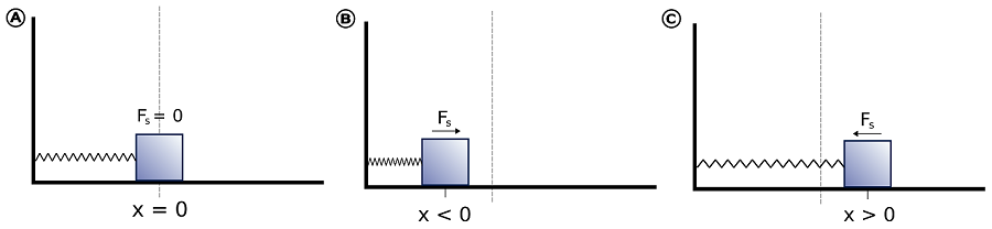
Figure 1:Harmonic motion governed by Hooke’s law. Any deviation from the equilibrium position is met with a restoring force, and in the absence of friction the bead oscillates indefinitely about equilibrium.
This is Hooke’s law, where the minus sign indicates that the direction of the force is always toward restoring the equilibrium location.
The constant characterizes the stiffness of the spring and is called the spring constant.
Solving harmonic oscillator problem
The classical equation of motion for a one-dimensional simple harmonic oscillator with a particle of mass m attached to a spring having spring constant k generates mechanical waves.
The introduced constant will be seen as the frequency of oscillations. Note that the frequency is inversely proportional to mass (heavier objects with the same spring constant oscillate more slowly around equilibrium) and increases with the spring constant (stiffer springs increase oscillations around equilibrium for the same mass).
The differential equation is a simple second-order, linear ODE which can be solved by the standard trick of plugging in an exponential and converting the problem to an algebraic equation. The solution is
The two constants are: , the amplitude of oscillations, and , a constant specifying the initial position of the bead.
Source
import numpy as np
import matplotlib.pyplot as plt
from matplotlib.animation import FuncAnimation
from IPython.display import HTML

def sho_anim(m, k=1.0, A=0.9, phi=0.0, duration=4.0, fps=30):
    ω = np.sqrt(k/m)
    t = np.linspace(0, duration, int(fps*duration))
    x = A*np.sin(ω*t + phi)

    fig, axes = plt.subplots(1, 2, figsize=(8, 2.5))
    ax_mass, ax_wave = axes

    # --- left: oscillating mass ---
    ax_mass.set_xlim(-1.2, 1.2)
    ax_mass.set_ylim(-0.5, 0.5)
    ax_mass.axis("off")
    ax_mass.set_title(f"Mass–Spring (m={m:g})")
    (mass_point,) = ax_mass.plot([], [], "o", ms=12)
    (trace_line,) = ax_mass.plot([], [], lw=2)

    # --- right: sinusoidal wave ---
    ax_wave.set_xlim(0, duration)
    ax_wave.set_ylim(-1.2*A, 1.2*A)
    ax_wave.set_xlabel("time t")
    ax_wave.set_ylabel("x(t)")
    ax_wave.grid(True, ls="--", alpha=0.4)
    ax_wave.set_title("x(t) = A sin (ωt + φ)")
    (wave_line,) = ax_wave.plot([], [], lw=2)
    (wave_point,) = ax_wave.plot([], [], "o")

    def init():
        for line in (mass_point, trace_line, wave_line, wave_point):
            line.set_data([], [])
        return mass_point, trace_line, wave_line, wave_point

    def update(i):
        xi = x[i]
        mass_point.set_data([xi], [0])
        trace_line.set_data(x[:i+1], np.zeros(i+1))
        wave_line.set_data(t[:i+1], x[:i+1])
        wave_point.set_data([t[i]], [xi])
        return mass_point, trace_line, wave_line, wave_point

    return FuncAnimation(fig, update, init_func=init, frames=len(t), interval=1000/fps, blit=True)

# --- Two animations: normal mass and heavier mass ---
anim1 = sho_anim(m=1.0, duration=10.0)
anim2 = sho_anim(m=10.0, duration=10.0)  # slower oscillation

# Inline display in Jupyter / Jupyter Book
plt.close()  # Prevents static display of the last frame
HTML(anim1.to_jshtml() + "<br><hr><br>" + anim2.to_jshtml())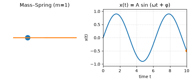
Energy of the harmonic oscillator
In classical mechanics, when we have a conservative system (no friction, energy conserved) the force is the gradient of a potential energy
This means the steeper the potential, the larger the force, and the minus sign indicates that the force restores the system to its equilibrium position.
The potential energy can be obtained by integrating:
Thus the potential energy for a simple harmonic oscillator is a parabolic function of displacement. It is convenient to set and measure potential energy relative to the equilibrium state .
The total energy, consisting of kinetic and potential energies, will be used to obtain the Schrodinger equation.
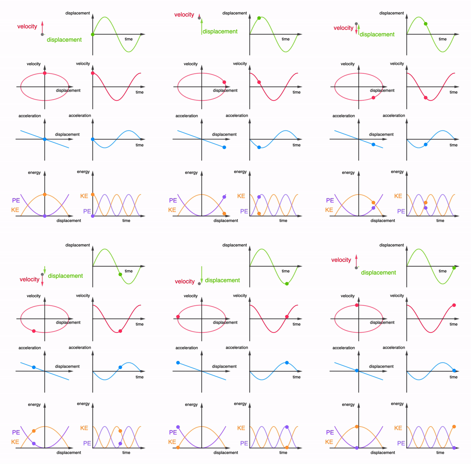
Figure 2:A harmonic oscillator in vacuum is conservative: kinetic and potential energy interconvert with no total energy dissipated into the environment. Position , velocity , and acceleration all oscillate at the same constant frequency but with different amplitudes.
Diatomic molecules and two-body problem
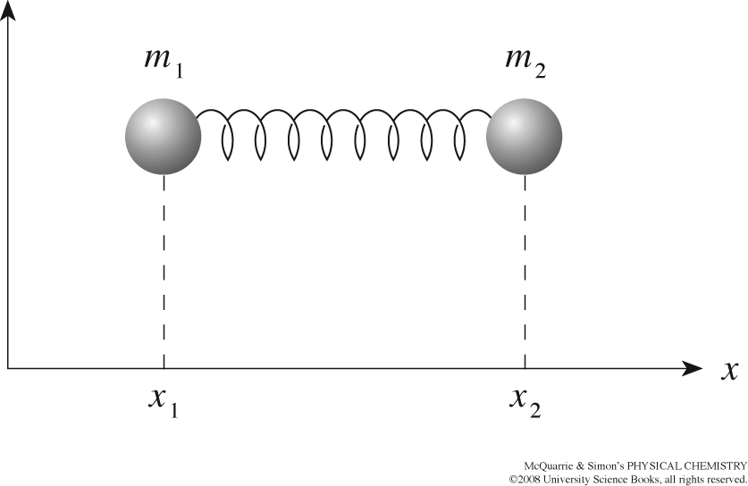
Figure 3:We can reduce the two-body problem of vibrating atoms to a one-body problem of a single particle with an effective reduced mass , so .
Derivation
Equations of motion for diatomic molecule modeled as beads bound by a spring are:
where , a reflection of Newton’s third law. By introducing more convenient coordinates in the form of the relative distance and the center of mass , we now reduce the two-body problem to a one-body problem.
The diatomic molecule is stable because the same force acts on both ends
By expressing the equations of motion in terms of the center of mass, we find that the center of mass moves freely without acceleration.
Next, by taking the difference between the coordinates and , we express the equations of motion in terms of the relative distance
This equation looks identical to the problem of a bead anchored to a wall with a spring. We have thus managed to reduce the two-body problem to a one-body problem by replacing the masses of the bodies with a reduced mass , so
### Beads and springs model of molecules

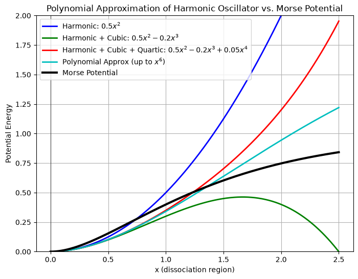
- Before discussing the harmonic oscillator approximation, let us reflect on when it is a good approximation and under which circumstances it breaks down. For an arbitrary potential energy function of $x$, we can carry out a Taylor expansion around the equilibrium bond length $x_0$, obtaining an infinite series.

$$U(x) = U(x_0)+U'(x_0)(x-x_0)+\frac{1}{2!}U''(x_0)(x-x_0)^2+\frac{1}{3!}U'''(x_0)(x-x_0)^3+...$$


:::{figure} images/harm_approx.png
:label: fig-classical-harmonic-oscillator-4
:alt: harmls
:width: 300px

Deviation of the true potential (blue) from the simple harmonic approximation (red), with the cubic correction shown in green.
Setting the energy scale relative to and recognizing that the first derivative vanishes at the minimum , we have
Hence we see that the harmonic approximation keeps only the first non-vanishing term! Furthermore, the spring constant and the subsequent anharmonicity constants such as are higher-order derivatives of the potential energy. That is, the more nonlinear the potential, the larger the contribution of these terms. Conversely, the closer the potential is to a quadratic form, the more accurate the harmonic assumption.
Source
import numpy as np
import matplotlib.pyplot as plt

# Define the range for x values, focusing on the dissociation region
x = np.linspace(0, 2.5, 500)

# Define the harmonic potential (quadratic term)
harmonic = 0.5 * x**2

# Define the harmonic + cubic potential
harmonic_cubic = 0.5 * x**2 - 0.2 * x**3

# Define the harmonic + cubic + quartic potential
harmonic_cubic_quartic = 0.5 * x**2 - 0.2 * x**3 + 0.05 * x**4

# Define the harmonic + cubic + quartic + higher-order polynomial (5th and 6th order)
polynomial_approx = 0.5 * x**2 - 0.2 * x**3 + 0.05 * x**4 - 0.01 * x**5 + 0.001 * x**6

# Define the Morse potential
def morse_potential(x, D=1, a=1):
    return D * (1 - np.exp(-a * x))**2

# Set parameters for Morse potential
D = 1  # Depth of the potential well
a = 1  # Width of the potential well

# Compute Morse potential
morse = morse_potential(x, D, a)

# Plot all the potentials, showing progression
plt.figure(figsize=(8, 6))

# Harmonic only
plt.plot(x, harmonic, label='Harmonic: $0.5  x^2$', color='b', lw=2)

# Harmonic + Cubic
plt.plot(x, harmonic_cubic, label='Harmonic + Cubic: $0.5  x^2 - 0.2  x^3$', color='g', lw=2)

# Harmonic + Cubic + Quartic
plt.plot(x, harmonic_cubic_quartic, label='Harmonic + Cubic + Quartic: $0.5  x^2 - 0.2  x^3 + 0.05  x^4$', color='r', lw=2)

# Polynomial approximation (up to 6th order)
plt.plot(x, polynomial_approx, label='Polynomial Approx (up to $x^6$)', color='c', lw=2)

# Morse potential
plt.plot(x, morse, label='Morse Potential', color='k', lw=3)

# Add labels and legend
plt.title('Polynomial Approximation of Harmonic Oscillator vs. Morse Potential')
plt.xlabel('x (dissociation region)')
plt.ylabel('Potential Energy')
plt.axhline(0, color='black',linewidth=0.5)
plt.axvline(0, color='black',linewidth=0.5)
plt.grid(True)
plt.legend()
plt.ylim([0, 2])
(0.0, 2.0)